1D Speckle Generation & Analysis
Scott Prahl
A speckle pattern is the irradiance produced when coherent light scatters from a rough surface: many randomly phased wavelets interfere, and the result is a grainy pattern of bright and dark regions.
This notebook covers
fully developed speckle, polarized and unpolarized, and
partially developed speckle, where the surface is too smooth to randomize the phase completely.
Speckle irradiance is exponentially distributed and never negative. That is quite different from the correlated Gaussian sequences in the Correlated Random Sequences notebook, which are sometimes mistaken for speckle because one of them is also named “exponential”. There the word describes the autocorrelation; here it describes the distribution of irradiance.
[1]:
%config InlineBackend.figure_format = 'retina'

import sys
import numpy as np
import matplotlib.pyplot as plt

if sys.platform == "emscripten":
    import piplite

    await piplite.install("pyspeckle")

import pyspeckle

# fix the seed so re-running this notebook reproduces the same figures
np.random.seed(0)
Fully developed speckle
When the surface roughness is much larger than the wavelength, the scattered phase is uniformly distributed over \(2\pi\) and the speckle is fully developed. create_exponential(M, pix_per_speckle) builds this directly: uniform random phase across an aperture, Fourier transformed, magnitude squared.
pix_per_speckle sets the sampling. A value of 2 is the Nyquist limit, 8 gives eight pixels across the smallest speckle.
[2]:
M = 2048
speckle = pyspeckle.create_exponential(M, 8)

plt.plot(speckle, ".", markersize=2)
plt.xlabel("Position (pixels)")
plt.ylabel("Irradiance")
plt.title("Fully developed speckle, contrast K=%.2f" % (np.std(speckle) / np.mean(speckle)))
plt.show()

The irradiance is exponentially distributed
For fully developed polarized speckle the probability density of the irradiance is
so the most likely value is zero – dark points are the most common. The speckle contrast, the ratio of standard deviation to mean, is exactly one.
[3]:
speckle = pyspeckle.create_exponential(100000, 4)
mean = np.mean(speckle)

count, bins, ignored = plt.hist(speckle, 40, density=True)
plt.plot(bins, np.exp(-bins / mean) / mean, "k", lw=2)
plt.xlabel("Irradiance")
plt.ylabel("Probability Density Function")
plt.title("Exponential distribution, K=%.3f (theory 1)" % (np.std(speckle) / mean))
plt.show()

Speckle size
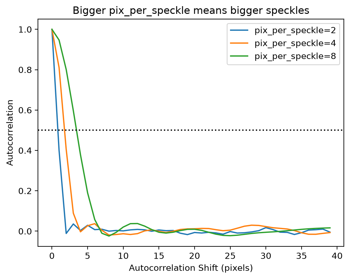
The speckle size is set by the aperture, and pix_per_speckle controls how finely it is sampled. The autocorrelation width grows in proportion.
[4]:
for pix_per_speckle in [2, 4, 8]:
    speckle = pyspeckle.create_exponential(16384, pix_per_speckle)
    ac = pyspeckle.autocorrelation(speckle)
    plt.plot(ac[:40], label="pix_per_speckle=%d" % pix_per_speckle)

plt.axhline(0.5, color="black", ls=":")
plt.xlabel("Autocorrelation Shift (pixels)")
plt.ylabel("Autocorrelation")
plt.title("Bigger pix_per_speckle means bigger speckles")
plt.legend()
plt.show()
All the statistics at once
statistics_plot collects the useful views into one figure: the trace, the probability density of the irradiance, the power spectral density, and that same density on a log scale, where a fully developed pattern is a straight line.
The power spectral density is the frequency-domain counterpart of the autocorrelation above. It cuts off at \(1/\mathtt{pix\_per\_speckle}\), so at 8 pixels per speckle the energy is confined within \(\pm0.125\) cycles per pixel. Sampling at Nyquist would push that cutoff out to the edge of the plot.
[5]:
speckle = pyspeckle.create_exponential(8192, 8)
pyspeckle.statistics_plot(speckle)
# theoretical exponential PDF over both histogram panels
g = np.linspace(0, speckle.max(), 200)
pdf = np.exp(-g / speckle.mean()) / speckle.mean()
plt.subplot(222)
plt.plot(g, pdf, "r", lw=2)
plt.subplot(224)
plt.semilogy(g, pdf, "r", lw=2)

plt.show()

Polarized and unpolarized speckle
Unpolarized light is the incoherent sum of two independent speckle patterns, one per polarization state. Adding two exponentials gives a gamma distribution with shape 2, and the contrast drops from 1 to \(1/\sqrt{2}\).
create_unpolarized is exactly create_exponential(..., polarization=0).
[6]:
M = 100000
polarized = pyspeckle.create_exponential(M, 4)
unpolarized = pyspeckle.create_unpolarized(M, 4)

for data, label in [(polarized, "polarized"), (unpolarized, "unpolarized")]:
    K = np.std(data) / np.mean(data)
    plt.hist(data / np.mean(data), 60, density=True, histtype="step", lw=2, label="%s, K=%.3f" % (label, K))

plt.xlabel("Irradiance / mean")
plt.ylabel("Probability Density Function")
plt.title("Theory: K=1 polarized, K=%.3f unpolarized" % (1 / np.sqrt(2)))
plt.xlim(0, 5)
plt.legend()
plt.show()

Local contrast
Speckle contrast is the standard deviation divided by the mean. Measured over a whole pattern it is a single number, but it is often more useful measured over a sliding window, because the window follows variation along the trace.
local_contrast(x, kernel) returns both: the contrast at every window position and the contrast of the whole trace. Only valid window positions are returned, so for an M-long trace and an N-long kernel there are M-N+1 values and none of them are contaminated by the ends.
The window has to hold enough speckles
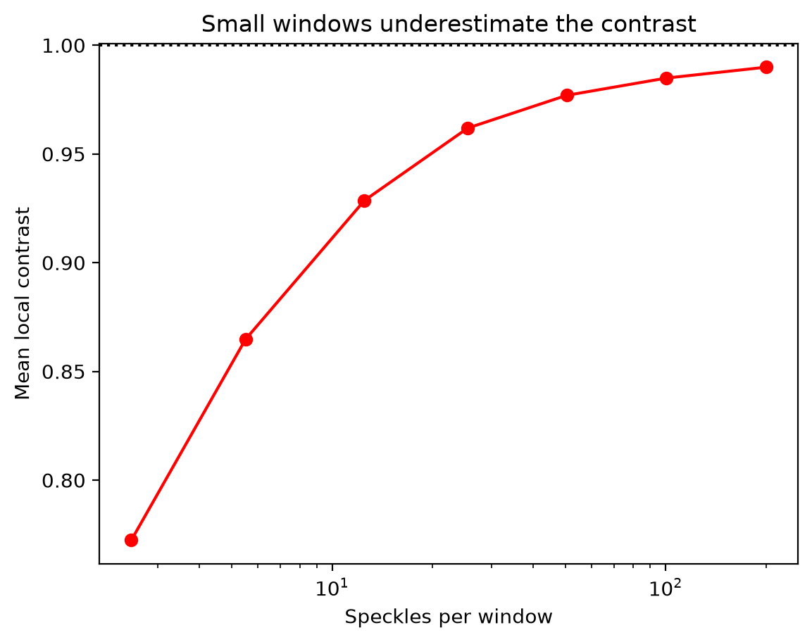
A window covering only a few speckles gives a noisy estimate, and one that is still biased low even though the variance is computed the unbiased way: the contrast of a handful of correlated samples underestimates the true value. The estimate creeps up toward the global contrast of 1 as the window grows.
This is the single most common way to get local speckle contrast wrong, so it is worth seeing the size of the effect.
[7]:
speckle = pyspeckle.create_exponential(16384, 2)
print("global contrast K = %.3f" % (np.std(speckle) / np.mean(speckle)))
print()
print("  window   speckles   mean C   spread")
windows = [5, 11, 25, 51, 101, 201, 401]
means = []
for n in windows:
    C, K = pyspeckle.local_contrast(speckle, np.ones(n))
    means.append(np.mean(C))
    print("  %6d   %8.1f   %6.3f   %6.3f" % (n, n / 2, np.mean(C), np.std(C)))

plt.semilogx(np.array(windows) / 2, means, "ro-")
plt.axhline(1.0, color="black", ls=":")
plt.xlabel("Speckles per window")
plt.ylabel("Mean local contrast")
plt.title("Small windows underestimate the contrast")
plt.show()
global contrast K = 0.994

  window   speckles   mean C   spread
       5        2.5    0.772    0.248
      11        5.5    0.865    0.209
      25       12.5    0.929    0.172
      51       25.5    0.962    0.137
     101       50.5    0.977    0.106
     201      100.5    0.985    0.078
     401      200.5    0.990    0.058
Putting it together
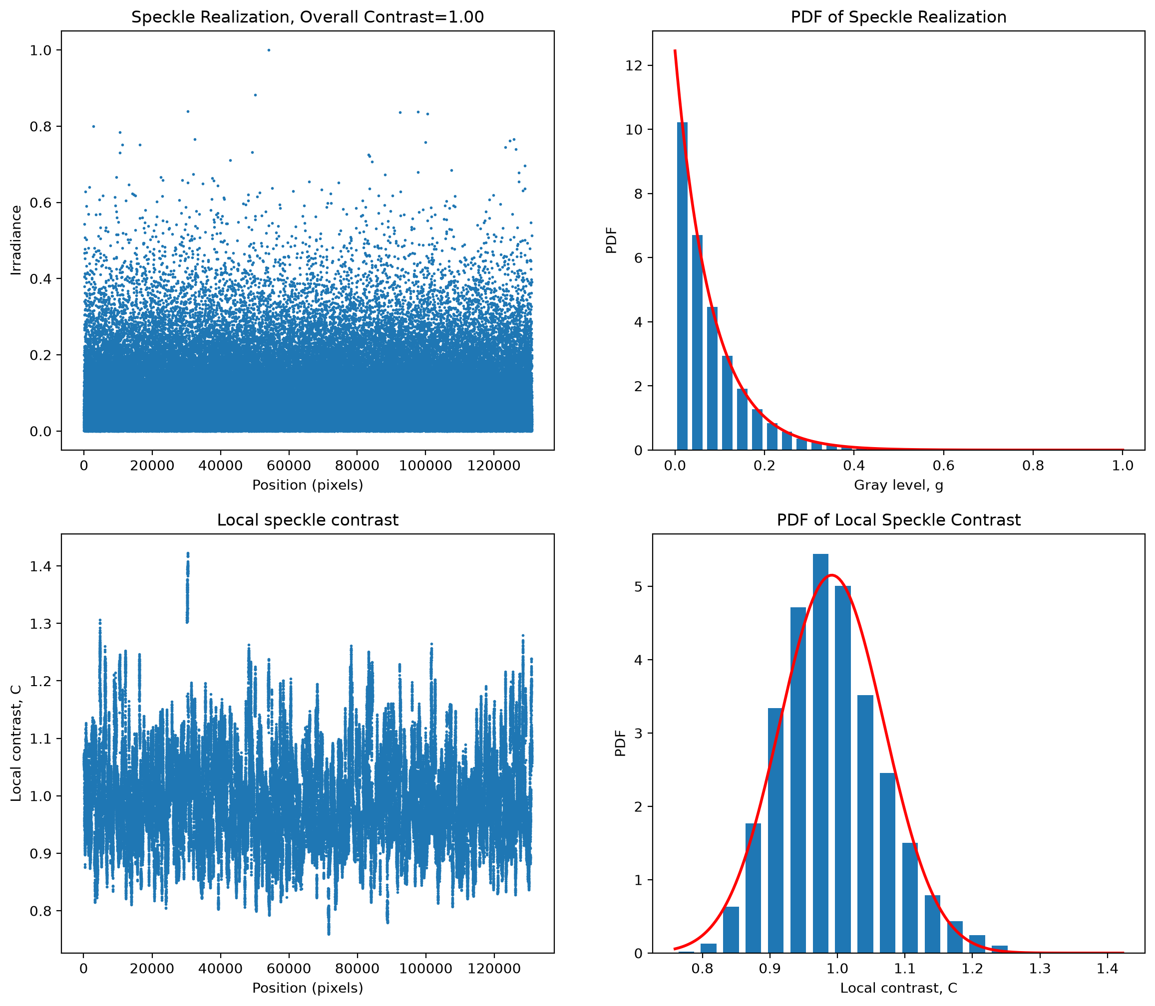
local_contrast_plot draws the trace, the local contrast, and the distribution of each. The contrast trace is plotted against the centre of its window so the two left panels share a position axis.
Here the window is 201 pixels at 2 pixels per speckle, about 100 speckles, so from the table above the local contrast should sit near 0.99.
[8]:
M, pix_per_speckle, n = 131072, 2, 201

speckle = pyspeckle.create_exponential(M, pix_per_speckle)
kernel = np.ones(n)
pyspeckle.local_contrast_plot(speckle, kernel)

# theoretical exponential PDF over the speckle histogram
plt.subplot(222)
g = np.linspace(0, speckle.max(), 200)
plt.plot(g, np.exp(-g / speckle.mean()) / speckle.mean(), "r", lw=2)

# gaussian fit over the local-contrast histogram
plt.subplot(224)
C, _ = pyspeckle.local_contrast(speckle, kernel)
c = np.linspace(C.min(), C.max(), 200)
plt.plot(c, np.exp(-((c - C.mean()) ** 2) / (2 * C.std() ** 2)) / (C.std() * np.sqrt(2 * np.pi)), "r", lw=2)

plt.show()
Phase screens
A phase screen is the phase a rough surface imposes on the light it reflects. create_phase_screen(M, sigma, cl, shape) generates one: a zero-mean Gaussian random process measured in radians, with standard deviation sigma and correlation length cl pixels.
It is worth being clear about what the arguments do, because the screen is an input to a scattering calculation rather than a speckle pattern:
sigma– how far the phase wanders, in radians. This sets how much light is scattered.cl– how quickly the phase varies along the surface, in pixels.shape–'gaussian'or'exponential'autocorrelation.
[9]:
M = 4096

plt.subplots(1, 2, figsize=(13, 4.5))

plt.subplot(1, 2, 1)
for sigma in [0.5, 2.0, 8.0]:
    plt.plot(pyspeckle.create_phase_screen(M, sigma, 16)[:400], label="sigma=%.1f" % sigma)
plt.xlabel("Position (pixels)")
plt.ylabel("Phase (radians)")
plt.title("sigma sets how far the phase wanders")
plt.legend()

plt.subplot(1, 2, 2)
for cl in [4, 16, 64]:
    plt.plot(pyspeckle.create_phase_screen(M, 1.0, cl)[:400], label="cl=%d" % cl)
plt.xlabel("Position (pixels)")
plt.ylabel("Phase (radians)")
plt.title("cl sets how quickly it varies")
plt.legend()

plt.show()

The correlation shape
correlation chooses between \(\exp(-x^2/c_l^2)\) and \(\exp(-x/c_l)\). The exponential form drops sharply at first and then has a long tail; the Gaussian form stays flat near zero lag and then falls away quickly.
The screen reproduces whichever is asked for, which is worth checking since the correlation is the whole point of the routine.
[10]:
M, cl = 32768, 16
lag = np.arange(60)

for shape, theory, colour in [
    ("gaussian", np.exp(-((lag / cl) ** 2)), "blue"),
    ("exponential", np.exp(-lag / cl), "red"),
]:
    screen = pyspeckle.create_phase_screen(M, 1.0, cl, correlation=shape)
    ac = pyspeckle.autocorrelation(screen)
    plt.plot(lag, ac[: len(lag)], "o", color=colour, markersize=3, label=shape)
    plt.plot(lag, theory, "-", color=colour, lw=1)

plt.xlabel("Autocorrelation Shift (pixels)")
plt.ylabel("Autocorrelation")
plt.title("Points are measured, lines are theory (cl=%d)" % cl)
plt.legend()
plt.show()

Partially developed speckle
Everything above assumed the scattered phase is uniform over \(2\pi\). If the surface roughness is comparable to the wavelength that is no longer true: part of the light is scattered and part continues undeviated, and the speckle is only partially developed.
The phase screens from the previous section are exactly what is needed here.
How much light is scattered
The fraction of the field that continues undeviated is
A screen with \(\sigma=0.25\) radians leaves 94% of the light unscattered, while \(\sigma=3\) leaves essentially none.
[11]:
sigmas = np.linspace(0.05, 3, 40)
measured = []
for sigma in sigmas:
    screen = pyspeckle.create_phase_screen(32768, sigma, 8)
    measured.append(abs(np.mean(np.exp(1j * screen))) ** 2)

plt.plot(sigmas, measured, "ro", markersize=3, label="measured")
plt.plot(sigmas, np.exp(-(sigmas**2)), "b", label=r"$\exp(-\sigma^2)$")
plt.xlabel(r"Phase standard deviation $\sigma$ (radians)")
plt.ylabel("Unscattered fraction")
plt.title("Rough surfaces scatter more")
plt.legend()
plt.show()

From partially to fully developed
Illuminating an aperture with the screen and transforming to the far field gives the speckle pattern. For small sigma most of the energy stays in the undeviated spike at the centre and there is little speckle. As sigma grows the spike disappears and the pattern approaches the fully developed case that create_exponential produces directly.
[12]:
M, L, cl = 8192, 16384, 4

fig, axes = plt.subplots(1, 3, figsize=(15, 4))
for ax, sigma in zip(axes, [0.5, 2.0, 8.0]):
    screen = pyspeckle.create_phase_screen(L, sigma, cl)
    u = np.exp(1j * screen)
    u[M:] = 0  # aperture
    I = np.abs(np.fft.fftshift(np.fft.fft(u))) ** 2
    ax.plot(I / I.max(), ".", markersize=1)
    ax.set_title("sigma=%.1f, unscattered %.2f" % (sigma, np.exp(-(sigma**2))))
    ax.set_xlabel("Position (pixels)")
axes[0].set_ylabel("Irradiance / max")
plt.tight_layout()
plt.show()

The transition shows up in the statistics. Away from the undeviated spike the contrast and skew both fall toward the fully developed values of 1 and 2 as the surface roughens.
[13]:
M, L, cl = 8192, 16384, 4
print("  sigma   unscattered      K     skew")
for sigma in [0.5, 1.0, 2.0, 4.0, 8.0]:
    screen = pyspeckle.create_phase_screen(L, sigma, cl)
    u = np.exp(1j * screen)
    u[M:] = 0
    I = np.abs(np.fft.fftshift(np.fft.fft(u))) ** 2
    middle = len(I) // 2
    keep = np.ones(len(I), dtype=bool)
    keep[middle - 64 : middle + 64] = False  # drop the undeviated spike
    Ik = I[keep]
    skew = np.mean(((Ik - Ik.mean()) / Ik.std()) ** 3)
    print("  %5.1f      %6.3f    %6.2f   %6.2f" % (sigma, np.exp(-(sigma**2)), Ik.std() / Ik.mean(), skew))

reference = pyspeckle.create_exponential(65536, 4)
skew = np.mean(((reference - reference.mean()) / reference.std()) ** 3)
print("\n  fully developed reference: K=%.2f, skew=%.2f" % (np.std(reference) / np.mean(reference), skew))
  sigma   unscattered      K     skew
    0.5       0.779      2.97     5.07
    1.0       0.368      2.69     4.85
    2.0       0.018      2.05     3.86
    4.0       0.000      1.25     2.72
    8.0       0.000      0.99     2.00

  fully developed reference: K=0.99, skew=1.93
Summary
create_exponential– fully developed polarized speckle, exponential irradiance, contrast 1.create_unpolarized– the incoherent sum of two polarizations, gamma-2 irradiance, contrast \(1/\sqrt{2}\).create_phase_screen– the correlated Gaussian phase imposed by a rough surface, the starting point for partially developed speckle.local_contrast_1Dandlocal_contrast_plot– contrast over a sliding window.statistics_plot– trace, irradiance density, and power spectrum in one figure.
The correlated Gaussian sequences create_correlated and create_correlated are covered in the Correlated Random Sequences notebook. They are not speckle.