2D Speckle Generation & Analysis

Scott Prahl

Adapted from the SimSpeckle Matlab script package described in Donald D. Duncan, Sean J. Kirkpatrick, “Algorithms for simulation of speckle (laser and otherwise),” Proc. SPIE 6855, Complex Dynamics and Fluctuations in Biomedical Photonics V, 685505 (6 February 2008); https://doi.org/10.1117/12.760518

The notebook is organized as

1. apertures, which set the size and shape of the speckle,

2. fully developed speckle, polarized through unpolarized,

3. partially developed speckle, from a rough surface that does not fully randomize the phase, and

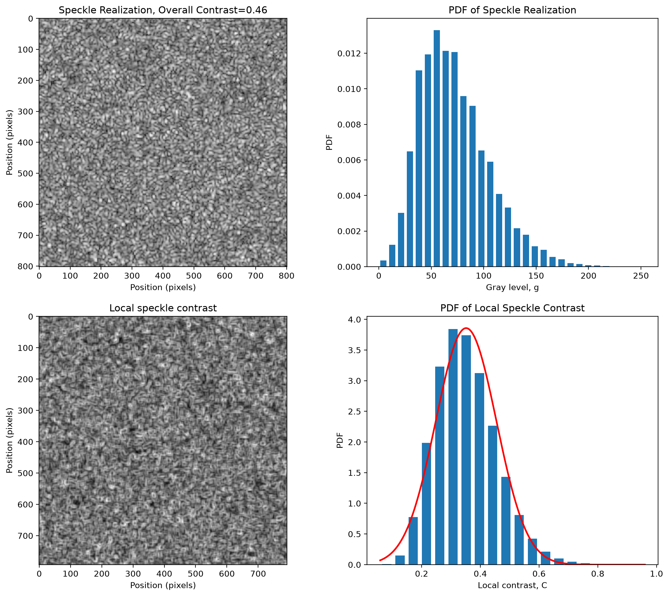
4. local contrast, measured over a sliding window.

%config InlineBackend.figure_format = 'retina'

import sys
import imageio
import numpy as np
import matplotlib.pyplot as plt

if sys.platform == "emscripten":
    import piplite

    await piplite.install("pyspeckle")

import pyspeckle

# fix the seed so re-running this notebook reproduces the same figures
np.random.seed(0)

if sys.platform == "emscripten":
    repo = "images/"
else:
    repo = "https://github.com/scottprahl/pyspeckle/raw/main/docs/images/"

Apertures set the speckle

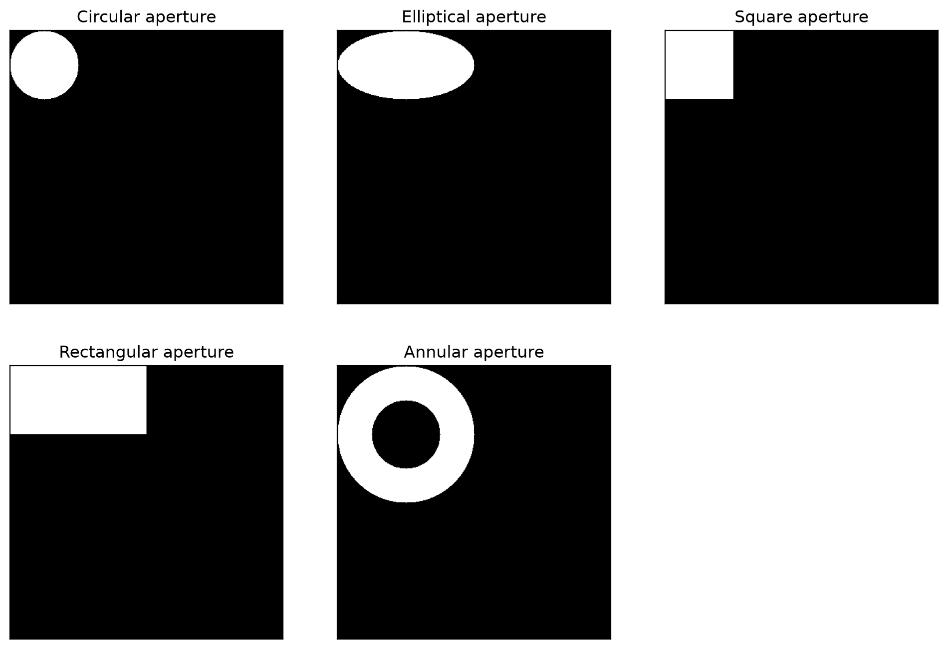
Speckle is produced by illuminating an aperture with randomly phased light and propagating to the far field. The aperture is not an implementation detail: its size fixes the speckle size, and its shape fixes the speckle shape. A wide aperture gives fine speckle, a narrow one gives coarse speckle, and an elongated aperture gives speckle elongated the other way.

pyspeckle builds the aperture with a private helper, _create_mask. It is not exported, but it is worth looking at first because everything else follows from it.

N, L, R = 400, 100, 50

plt.subplots(2, 3, figsize=(12, 8))
for i, (title, args, kwargs) in enumerate(
    [
        ("Circular", (N, R, R), {}),
        ("Elliptical", (N, L, R), {}),
        ("Square", (N, R, R), {"shape": "square"}),
        ("Rectangular", (N, L, R), {"shape": "square"}),
        ("Annular", (N, R, L), {"shape": "annulus"}),
    ]
):
    plt.subplot(2, 3, i + 1)
    plt.imshow(pyspeckle.core._create_mask(*args, **kwargs), cmap="gray")
    plt.title(title + " aperture")
    plt.xticks([])
    plt.yticks([])

plt.subplot(2, 3, 6)
plt.axis("off")
plt.show()

From aperture to speckle

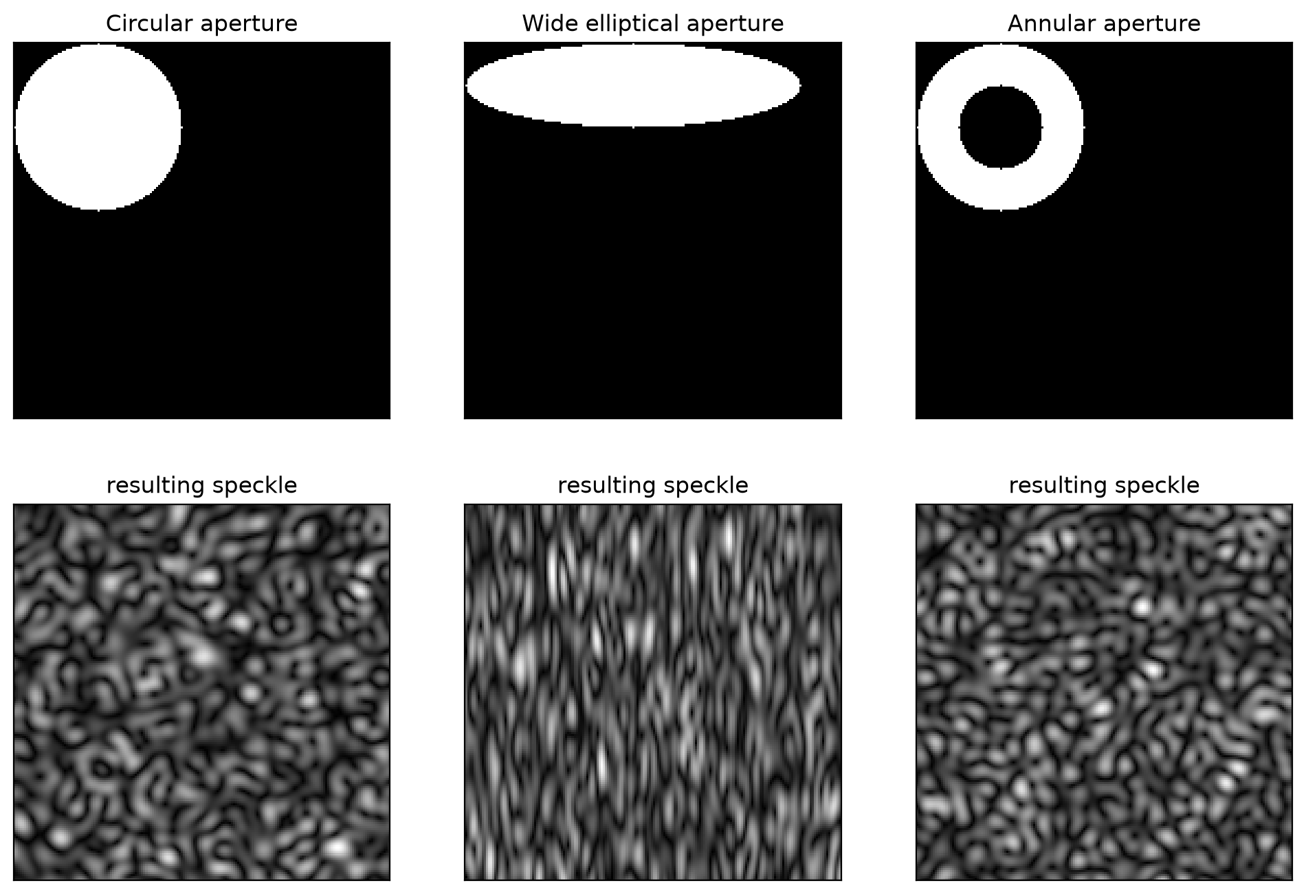
The recipe is short: fill the aperture with uniform random phase, Fourier transform, and take the squared magnitude. Doing it by hand shows how directly the aperture controls the result. A circular aperture gives round speckle; an aperture stretched horizontally gives speckle stretched vertically.

N = 512
apertures = [
    ("Circular", (N, 40, 40), {}),
    ("Wide elliptical", (N, 80, 20), {}),
    ("Annular", (N, 20, 40), {"shape": "annulus"}),
]

plt.subplots(2, 3, figsize=(12, 8))
for i, (title, args, kwargs) in enumerate(apertures):
    mask = pyspeckle.core._create_mask(*args, **kwargs)

    plt.subplot(2, 3, i + 1)
    plt.imshow(mask[:180, :180], cmap="gray")
    plt.title(title + " aperture")
    plt.xticks([])
    plt.yticks([])

    field = np.exp(1j * 2 * np.pi * np.random.rand(N, N)) * mask
    speckle = np.abs(np.fft.fftshift(np.fft.fft2(field))) ** 2

    plt.subplot(2, 3, i + 4)
    plt.imshow(np.sqrt(speckle[:180, :180]), cmap="gray")
    plt.title("resulting speckle")
    plt.xticks([])
    plt.yticks([])

plt.show()

Fully developed speckle

When the surface is rough compared with the wavelength the scattered phase is uniform over \(2\pi\) and the speckle is fully developed. The irradiance is exponentially distributed and the speckle contrast, the standard deviation divided by the mean, is one.

statistics_plot shows the pattern, its histogram, the power spectral density, and the same histogram on a log scale. The PSD reveals the sampling: when it fills the frame the pattern is at the Nyquist limit of two pixels per speckle.

Two pixels per speckle, the Nyquist limit

y = pyspeckle.create_exponential((201, 201), 2)
pyspeckle.statistics_plot(y)
# theoretical exponential PDF over both histogram panels
g = np.linspace(0, y.max(), 200)
pdf = np.exp(-g / y.mean()) / y.mean()
plt.subplot(222)
plt.plot(g, pdf, "r", lw=2)
plt.subplot(224)
plt.semilogy(g, pdf, "r", lw=2)

plt.show()

print("contrast K = %.3f (theory 1)" % (np.std(y) / np.mean(y)))

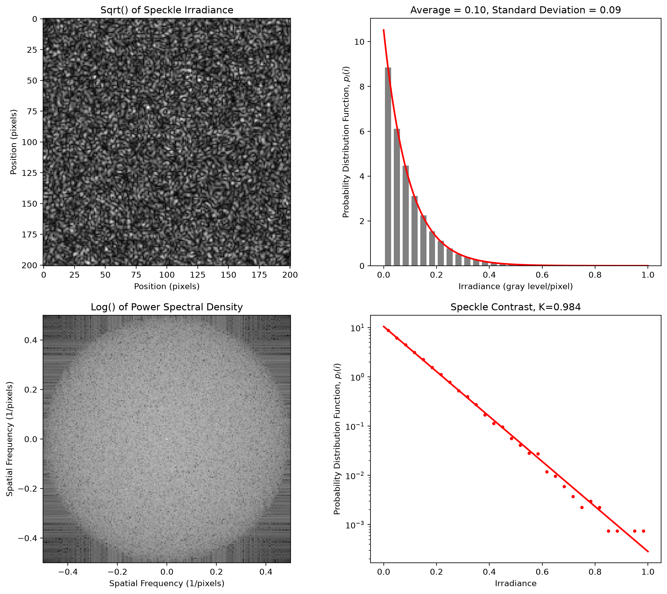
contrast K = 0.984 (theory 1)

Ten pixels per speckle

Increasing pix_per_speckle oversamples the same statistics: the speckles get visibly larger and the power spectral density shrinks to the middle of the frame. The contrast is unchanged, because contrast is a first-order statistic and does not depend on how finely the pattern is sampled.

The image does have to hold enough speckles for the measurement to settle. This one is about 20 speckles across, so roughly 400 in total, and the measured contrast lands within a few percent of 1. Coarser sampling would put fewer speckles in the same frame and the estimate would scatter more from one realization to the next.

y = pyspeckle.create_exponential((201, 201), 10)
pyspeckle.statistics_plot(y)
# theoretical exponential PDF over both histogram panels
g = np.linspace(0, y.max(), 200)
pdf = np.exp(-g / y.mean()) / y.mean()
plt.subplot(222)
plt.plot(g, pdf, "r", lw=2)
plt.subplot(224)
plt.semilogy(g, pdf, "r", lw=2)

plt.show()

print("contrast K = %.3f (unchanged by sampling)" % (np.std(y) / np.mean(y)))

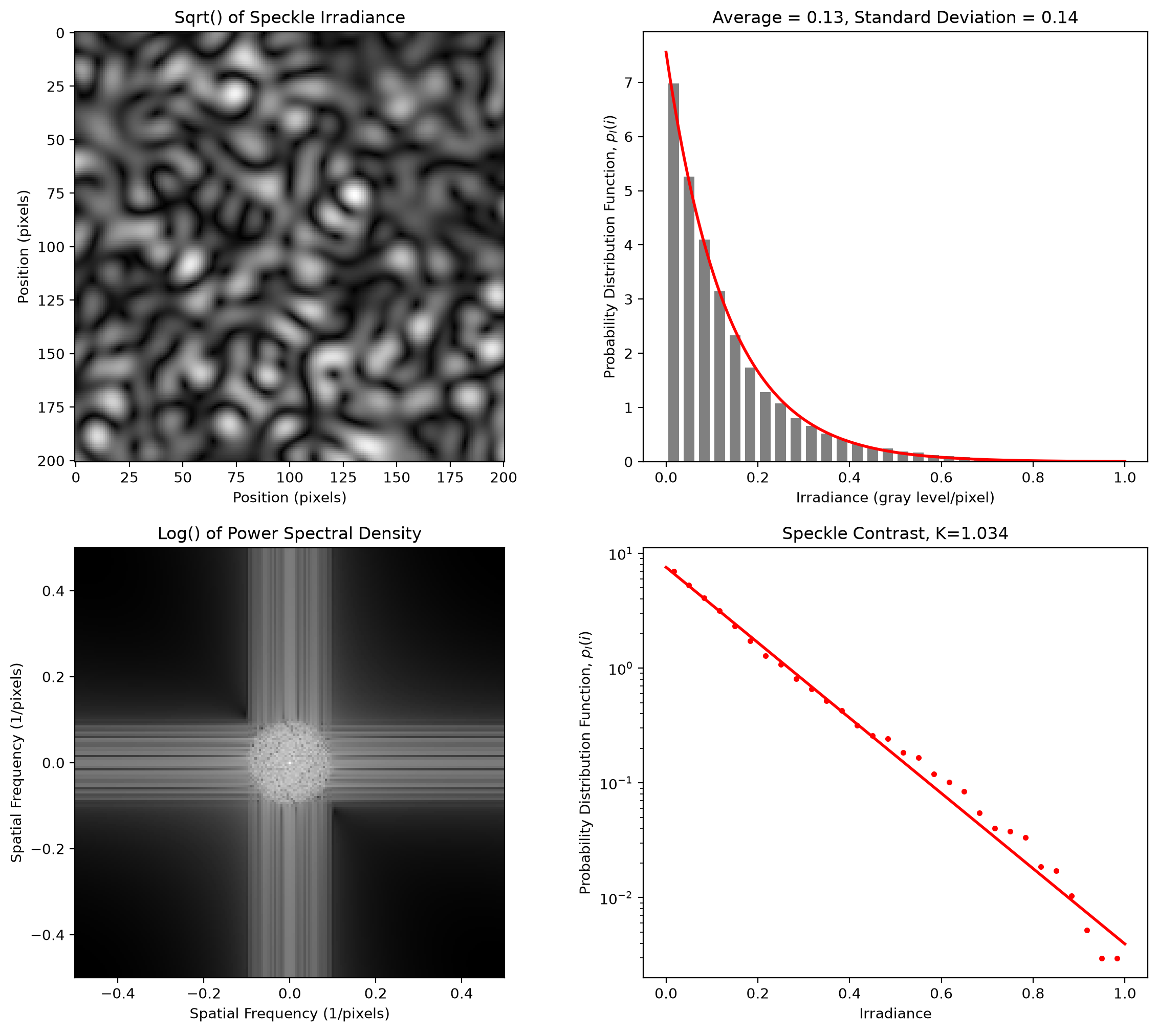
contrast K = 1.034 (unchanged by sampling)

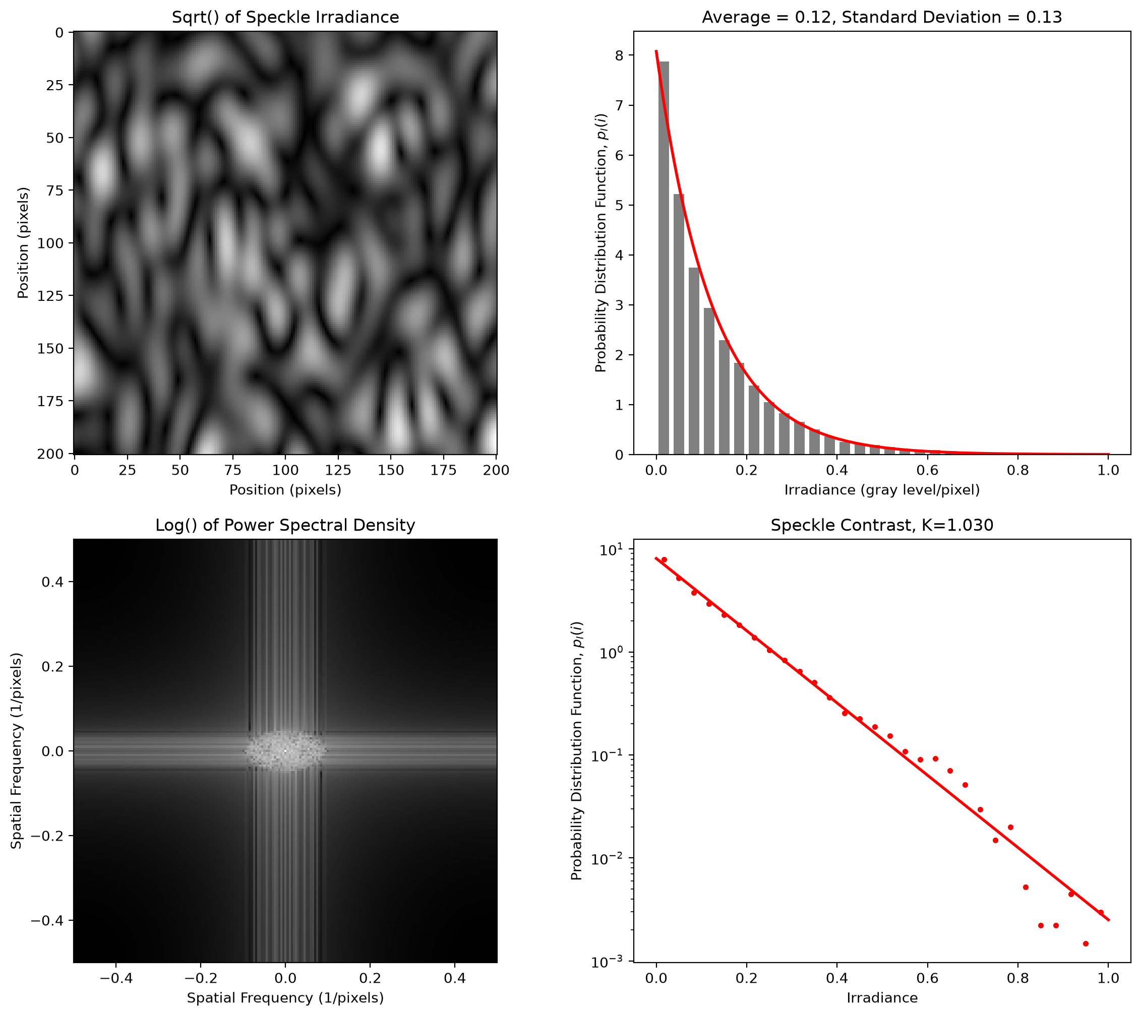
Anisotropic speckle

alpha is the ratio of horizontal to vertical speckle size. alpha=0.5 gives speckle that is twice as tall as it is wide.

y = pyspeckle.create_exponential((201, 201), 10, alpha=0.5)
pyspeckle.statistics_plot(y)
# theoretical exponential PDF over both histogram panels
g = np.linspace(0, y.max(), 200)
pdf = np.exp(-g / y.mean()) / y.mean()
plt.subplot(222)
plt.plot(g, pdf, "r", lw=2)
plt.subplot(224)
plt.semilogy(g, pdf, "r", lw=2)

plt.show()

Square and annular apertures

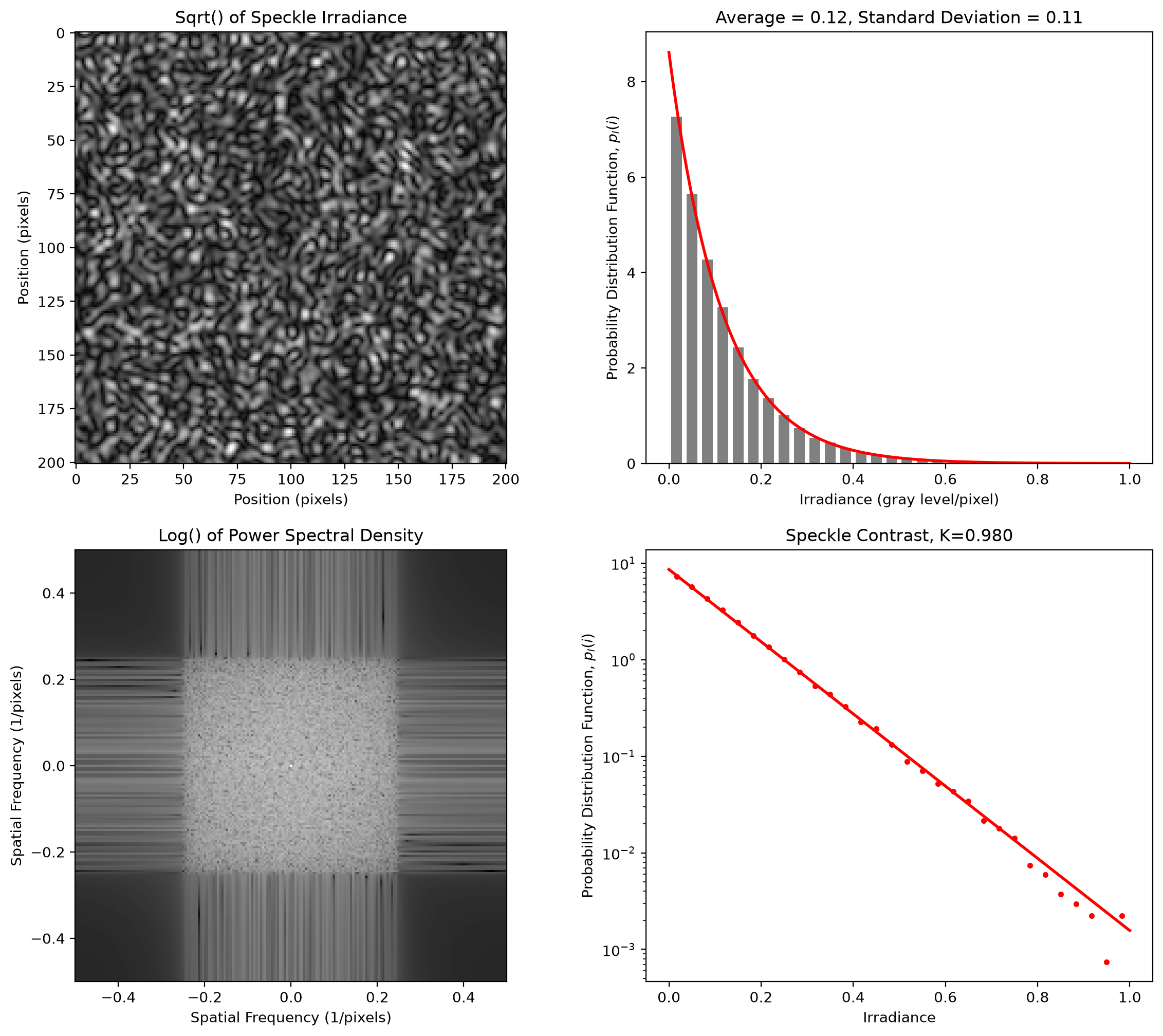
The aperture shape carries through to the speckle and to the power spectral density, which takes the shape of the aperture.

y = pyspeckle.create_exponential((201, 201), 4, aperture="square")
pyspeckle.statistics_plot(y)
# theoretical exponential PDF over both histogram panels
g = np.linspace(0, y.max(), 200)
pdf = np.exp(-g / y.mean()) / y.mean()
plt.subplot(222)
plt.plot(g, pdf, "r", lw=2)
plt.subplot(224)
plt.semilogy(g, pdf, "r", lw=2)

plt.show()

y = pyspeckle.create_exponential((201, 201), 4, aperture="annulus", alpha=3)
pyspeckle.statistics_plot(y)
# the aperture changes the speckle shape but not the irradiance distribution
g = np.linspace(0, y.max(), 200)
pdf = np.exp(-g / y.mean()) / y.mean()
plt.subplot(222)
plt.plot(g, pdf, "r", lw=2)
plt.subplot(224)
plt.semilogy(g, pdf, "r", lw=2)

plt.show()

Arbitrary apertures and modulated speckle

create_exponential builds the aperture for you, but only from a short list of named shapes. When the pupil is something else, build it yourself and hand it to create_from_aperture. Only the array matters, not where the opening sits inside it, because position adds a phase ramp that the magnitude squared throws away.

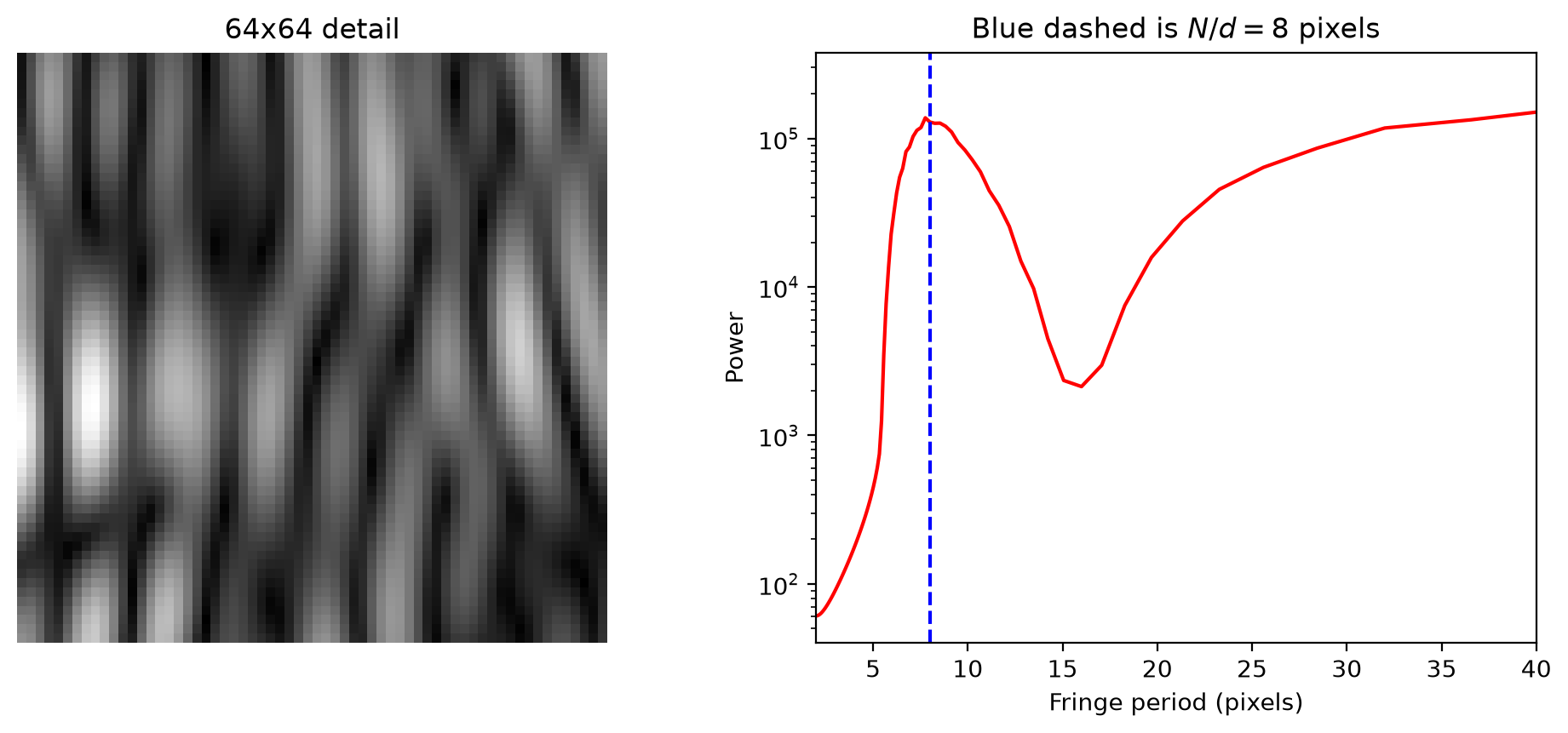
The interesting case is a pupil with two separated openings. Each opening alone gives ordinary speckle. Together they also interfere, and the speckle is crossed by Young’s fringes with period \(N/d\), where \(N\) is the width of the aperture array and \(d\) is the separation. Pushing the openings apart packs the fringes closer together, so the modulation is finer than the speckle grain it rides on.

def two_circles(N, separation, radius):
    """A pupil with two circular openings, separated along x."""
    y, x = np.ogrid[:N, :N]
    c = N // 2
    left = (x - c + separation / 2) ** 2 + (y - c) ** 2 <= radius**2
    right = (x - c - separation / 2) ** 2 + (y - c) ** 2 <= radius**2
    return left | right


M, N = 256, 1024
radius = 0.03 * N

plt.subplots(2, 2, figsize=(11, 11))
for col, separation in enumerate([0, N / 8]):
    aperture = two_circles(N, separation, radius)
    speckle = pyspeckle.create_from_aperture(aperture, (M, M))

    plt.subplot(2, 2, col + 1)
    #  the same crop for both, so the openings are drawn at the same scale
    half = int(N / 16 + 3 * radius)
    plt.imshow(aperture[N // 2 - half : N // 2 + half, N // 2 - half : N // 2 + half], cmap="gray")
    plt.title("one opening" if separation == 0 else "two openings, $d=N/8$")
    plt.axis("off")

    plt.subplot(2, 2, col + 3)
    plt.imshow(np.sqrt(speckle), cmap="gray")
    plt.title("speckle" if separation == 0 else "modulated speckle")
    plt.axis("off")

plt.show()

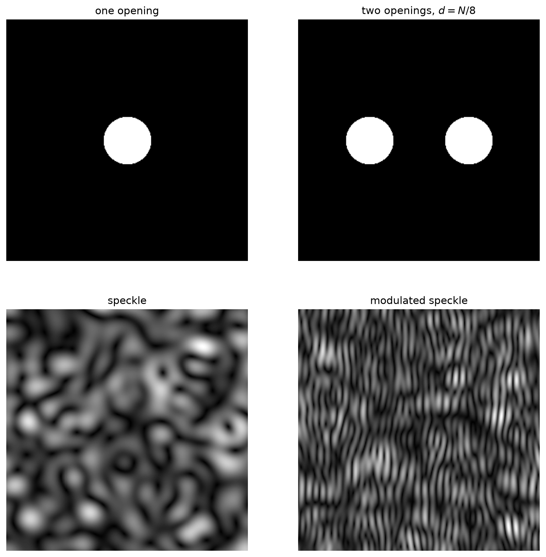
The two speckle patterns have the same grain, because the openings are the same size, but the right one is striped. A closer look at a small piece of it makes the fringes obvious, and averaging the power spectrum over many realizations puts their period exactly where the two-slit geometry predicts. The power rising again toward long periods is the speckle grain itself, which is coarser than the fringes riding on it.

separation = N / 8
speckle = pyspeckle.create_from_aperture(two_circles(N, separation, radius), (M, M))

plt.subplots(1, 2, figsize=(12, 4.5))
plt.subplot(121)
plt.imshow(np.sqrt(speckle[:64, :64]), cmap="gray")
plt.title("64x64 detail")
plt.axis("off")

# the fringes live at one spatial frequency, so the power spectrum finds them
power = np.zeros((M, M))
for _ in range(40):
    y = pyspeckle.create_from_aperture(two_circles(N, separation, radius), (M, M))
    power += np.abs(np.fft.fft2(y - y.mean())) ** 2
lobe = power.mean(axis=0)[: M // 2]

plt.subplot(122)
period = M / np.arange(1, M // 2)
plt.semilogy(period, lobe[1:], "r")
plt.axvline(N / separation, color="blue", ls="--")
plt.xlim(2, 40)
plt.xlabel("Fringe period (pixels)")
plt.ylabel("Power")
plt.title("Blue dashed is $N/d = %.0f$ pixels" % (N / separation))

plt.show()

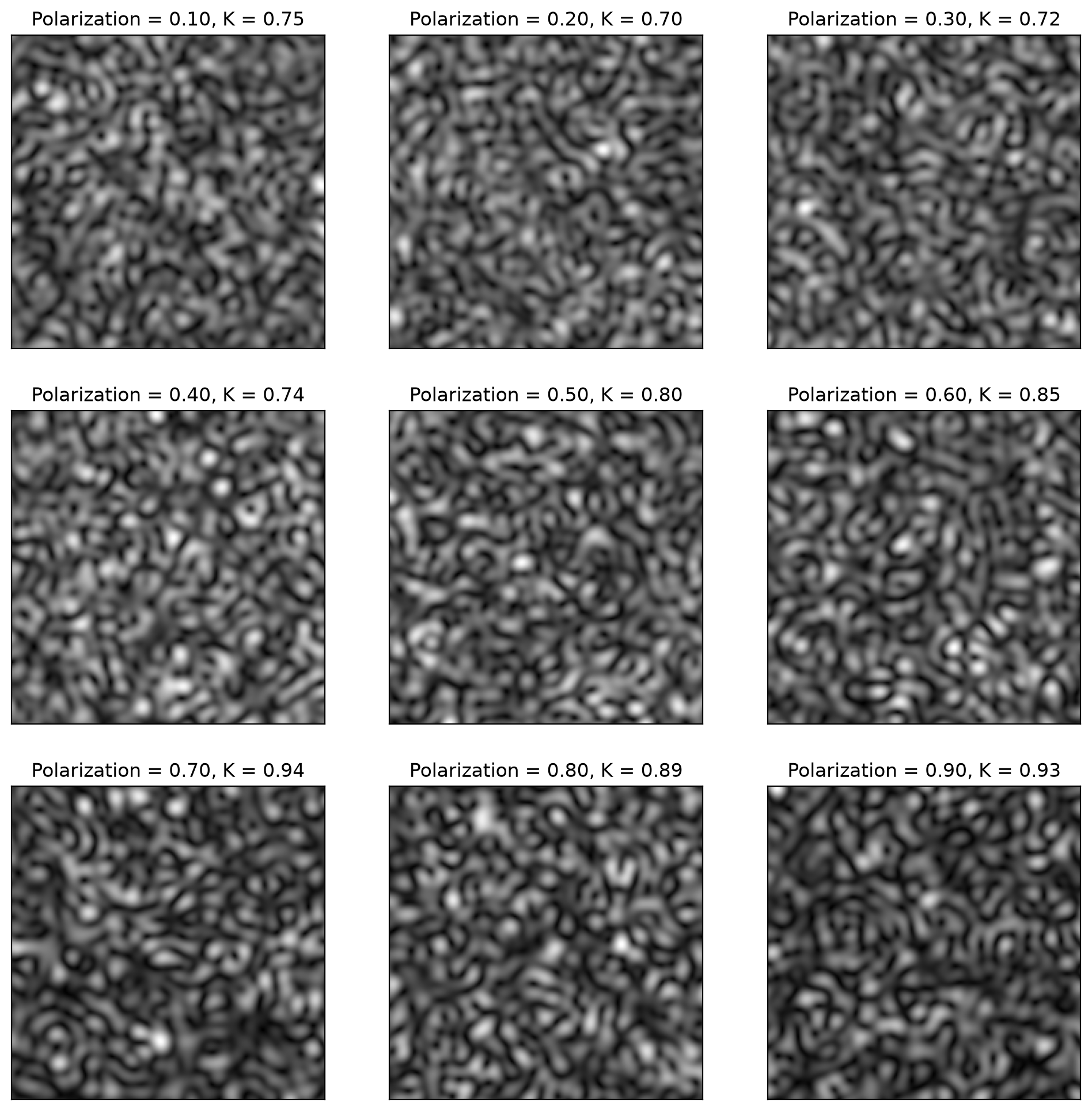
Degree of polarization

polarization=1 is fully polarized light with unit contrast. Lower values mix in a second, independent speckle pattern, and the contrast falls smoothly to \(1/\sqrt{2}\) at polarization=0.

plt.subplots(3, 3, figsize=(12, 12))
for i, pol in enumerate([0.1, 0.2, 0.3, 0.4, 0.5, 0.6, 0.7, 0.8, 0.9]):
    plt.subplot(3, 3, i + 1)
    y = pyspeckle.create_exponential((201, 201), 8, polarization=pol)
    plt.imshow(np.sqrt(y), cmap="gray")
    plt.title("Polarization = %.2f, K = %.2f" % (pol, np.std(y) / np.mean(y)))
    plt.xticks([])
    plt.yticks([])

plt.show()

Unpolarized speckle

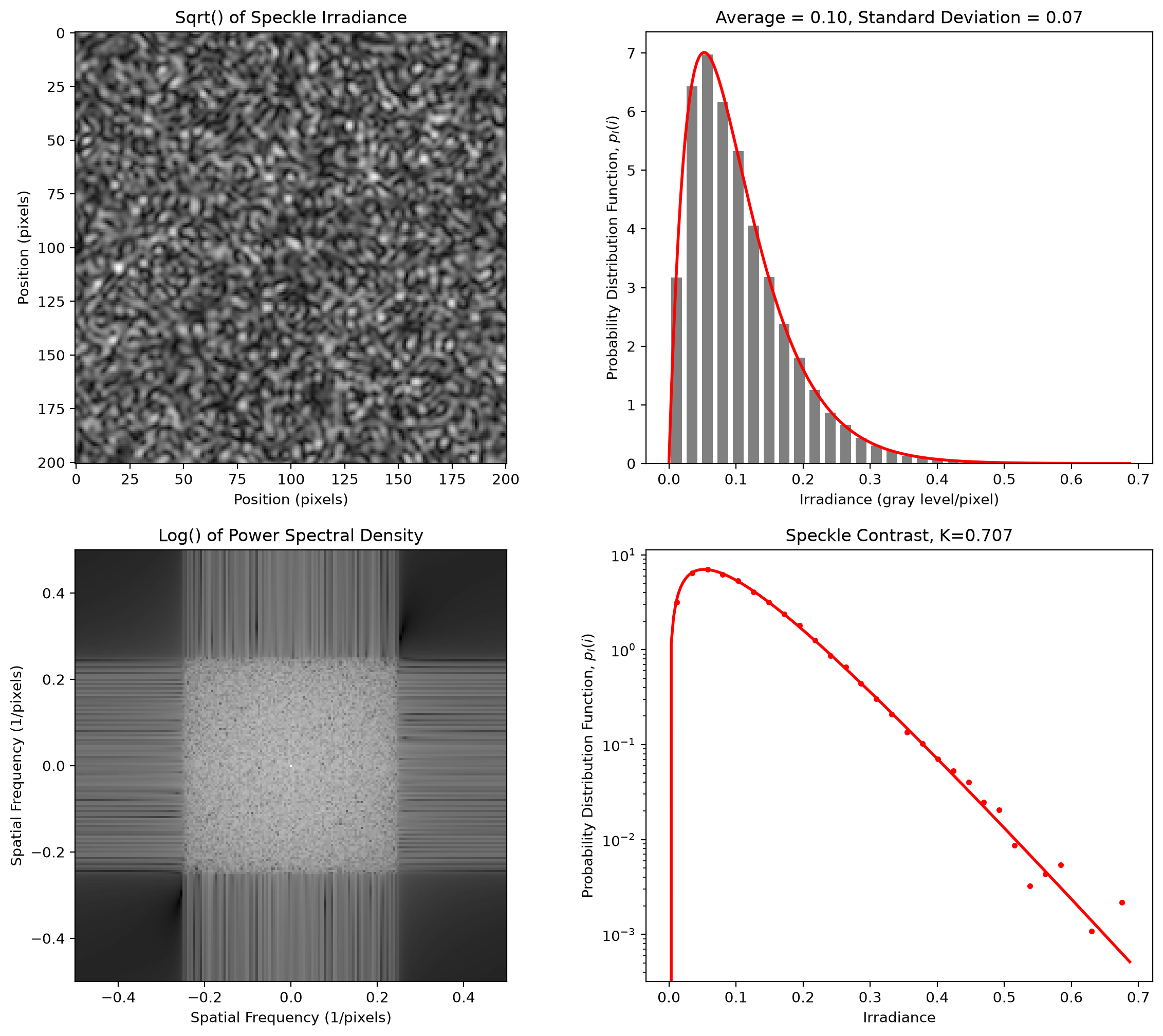
Unpolarized light adds two independent speckle patterns, one per polarization state. The irradiance follows a gamma distribution with shape 2 and the contrast is \(1/\sqrt{2}\approx0.707\). Duncan & Kirkpatrick call this the Rayleigh limit of zero polarization.

create_unpolarized is exactly create_exponential((..., ...), polarization=0).

y = pyspeckle.create_unpolarized((201, 201), 4, aperture="square")
pyspeckle.statistics_plot(y)
# unpolarized speckle adds two exponentials, so the theory is a gamma of shape 2
g = np.linspace(0, y.max(), 200)
scale = y.mean() / 2
pdf = g * np.exp(-g / scale) / scale**2
plt.subplot(222)
plt.plot(g, pdf, "r", lw=2)
plt.subplot(224)
plt.semilogy(g, pdf, "r", lw=2)

plt.show()

print("contrast K = %.3f (theory %.3f)" % (np.std(y) / np.mean(y), 1 / np.sqrt(2)))

contrast K = 0.707 (theory 0.707)

Partially developed speckle

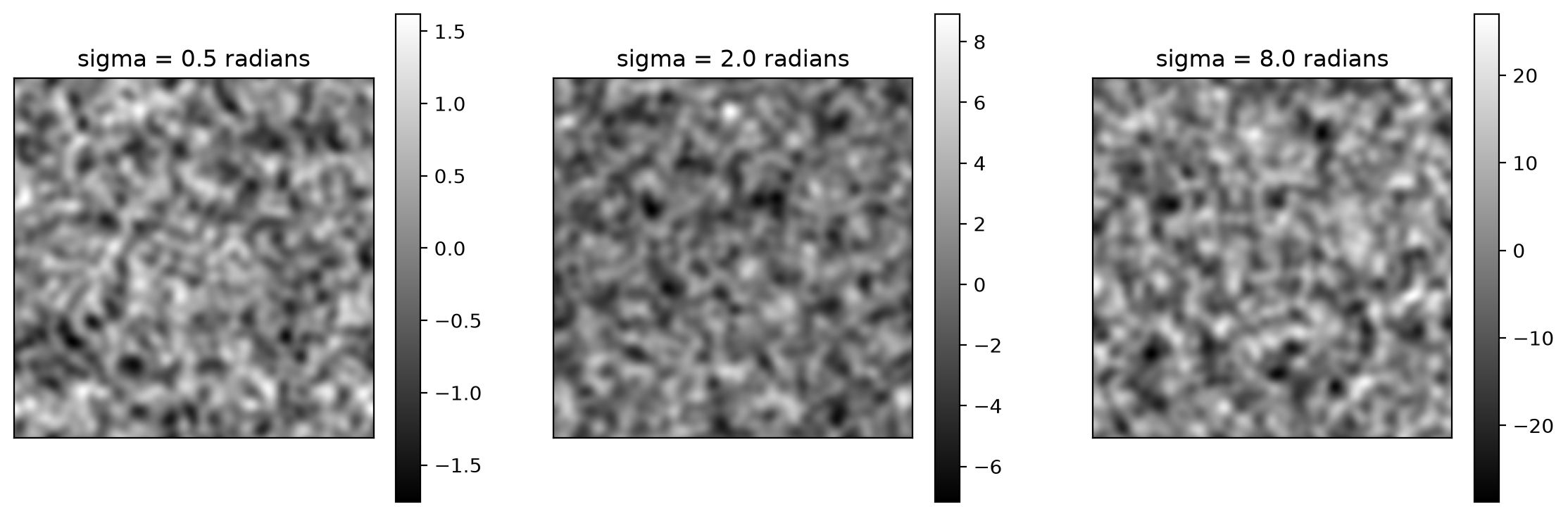
Everything above assumed a surface rough enough to spread the phase over \(2\pi\). A smoother surface leaves part of the light undeviated, and the speckle is only partially developed.

create_phase_screen((M, M), sigma, cl) generates the phase such a surface imposes: a zero-mean Gaussian random field of standard deviation sigma radians with correlation length cl pixels. The correlation is isotropic.

plt.subplots(1, 3, figsize=(14, 4.5))
for i, sigma in enumerate([0.5, 2.0, 8.0]):
    plt.subplot(1, 3, i + 1)
    screen = pyspeckle.create_phase_screen((256, 256), sigma, 8)
    plt.imshow(screen, cmap="gray")
    plt.title("sigma = %.1f radians" % sigma)
    plt.xticks([])
    plt.yticks([])
    plt.colorbar()

plt.show()

How much light is scattered

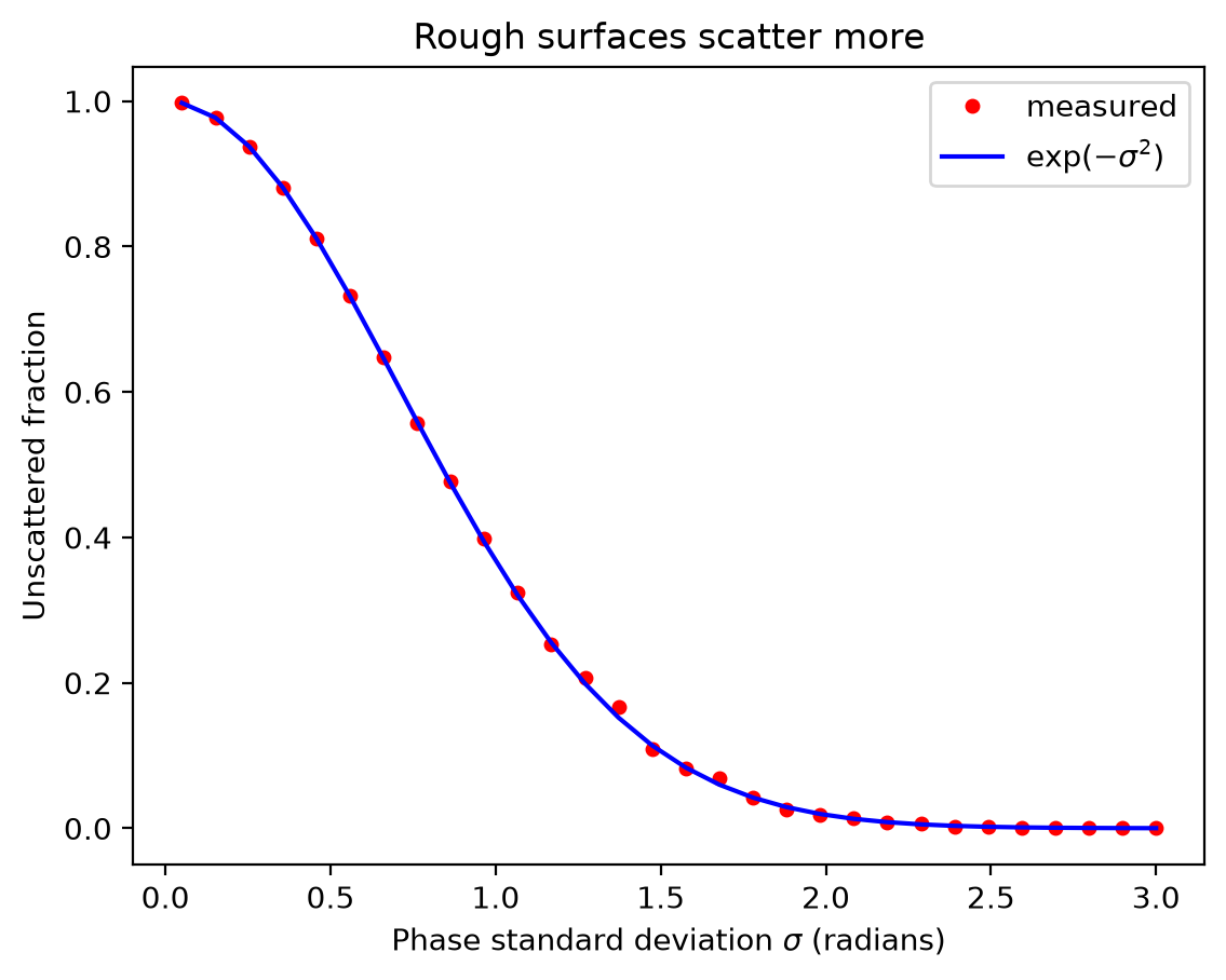
The fraction of the field left undeviated is

\[\left|\langle e^{i\phi}\rangle\right|^2 = e^{-\sigma^2}\]

so a screen with \(\sigma=0.5\) radians leaves 78% of the light unscattered while \(\sigma=3\) leaves essentially none.

sigmas = np.linspace(0.05, 3, 30)
measured = [abs(np.mean(np.exp(1j * pyspeckle.create_phase_screen((256, 256), s, 8)))) ** 2 for s in sigmas]

plt.plot(sigmas, measured, "ro", markersize=4, label="measured")
plt.plot(sigmas, np.exp(-(sigmas**2)), "b", label=r"$\exp(-\sigma^2)$")
plt.xlabel(r"Phase standard deviation $\sigma$ (radians)")
plt.ylabel("Unscattered fraction")
plt.title("Rough surfaces scatter more")
plt.legend()
plt.show()

From partially to fully developed

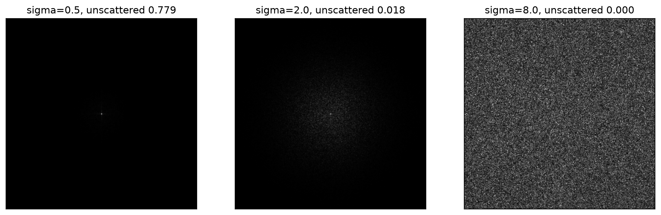
Illuminating an aperture with the screen and transforming gives the speckle. For small sigma most of the energy stays in the undeviated spike at the centre. As sigma grows the spike disappears and the statistics approach the fully developed values of \(K=1\) and skew \(=2\).

M, L, cl = 256, 512, 4

plt.subplots(1, 3, figsize=(14, 4.5))
for i, sigma in enumerate([0.5, 2.0, 8.0]):
    plt.subplot(1, 3, i + 1)
    u = np.exp(1j * pyspeckle.create_phase_screen((L, L), sigma, cl))
    u[M:, :] = 0
    u[:, M:] = 0
    speckle = np.abs(np.fft.fftshift(np.fft.fft2(u))) ** 2
    plt.imshow(np.sqrt(speckle), cmap="gray")
    plt.title("sigma=%.1f, unscattered %.3f" % (sigma, np.exp(-(sigma**2))))
    plt.xticks([])
    plt.yticks([])

plt.show()

M, L, cl = 256, 512, 4

print("  sigma   unscattered      K     skew")
for sigma in [0.5, 1.0, 2.0, 4.0, 8.0]:
    u = np.exp(1j * pyspeckle.create_phase_screen((L, L), sigma, cl))
    u[M:, :] = 0
    u[:, M:] = 0
    speckle = np.abs(np.fft.fftshift(np.fft.fft2(u))) ** 2

    middle = L // 2
    keep = np.ones(speckle.shape, dtype=bool)
    keep[middle - 16 : middle + 16, middle - 16 : middle + 16] = False  # drop the spike
    kept = speckle[keep]
    skew = np.mean(((kept - kept.mean()) / kept.std()) ** 3)
    print("  %5.1f      %7.3f  %7.2f  %7.2f" % (sigma, np.exp(-(sigma**2)), kept.std() / kept.mean(), skew))

reference = pyspeckle.create_exponential((256, 256), 4)
skew = np.mean(((reference - reference.mean()) / reference.std()) ** 3)
print("\n  fully developed reference: K=%.2f, skew=%.2f" % (np.std(reference) / np.mean(reference), skew))

  sigma   unscattered      K     skew
    0.5        0.779     7.32    21.57
    1.0        0.368     5.80    13.17
    2.0        0.018     3.48     7.74
    4.0        0.000     1.53     3.89
    8.0        0.000     1.00     2.02

  fully developed reference: K=1.01, skew=1.99

Boiling speckle

Everything so far has been a single frozen pattern. When the object moves, the speckle changes, and create_boiling_speckle produces that sequence.

A single random-phase screen is illuminated through a circular pupil and the pupil is translated one column per frame. This is the back focal plane geometry: the pattern seethes without appearing to travel, which is why it is described as boiling. Once the pupil has moved its own diameter the pattern has forgotten where it started.

The function returns the cube, the correlation of each frame with the first, and the correlation predicted by theory.

M = 128
cube, correlation, theory = pyspeckle.create_boiling_speckle((M, M), 2)

print("cube shape          ", cube.shape)
print("frames              ", cube.shape[2])
print("contrast of frame 0  %.3f" % (np.std(cube[:, :, 0]) / np.mean(cube[:, :, 0])))

cube shape           (128, 128, 129)
frames               129
contrast of frame 0  1.004

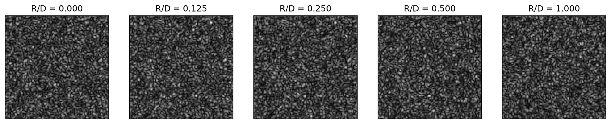
Each frame is an ordinary fully developed speckle pattern. Stepping through the cube shows the pattern reorganizing itself; by the last frame nothing of the first remains.

R/D below is the pupil displacement as a fraction of its diameter.

lags = [0, M // 8, M // 4, M // 2, M]

plt.subplots(1, len(lags), figsize=(15, 3.4))
for i, frame in enumerate(lags):
    plt.subplot(1, len(lags), i + 1)
    plt.imshow(np.sqrt(cube[:, :, frame]), cmap="gray", vmin=0, vmax=1)
    plt.title("R/D = %.3f" % (frame / M))
    plt.xticks([])
    plt.yticks([])

plt.show()

Decorrelation follows the aperture

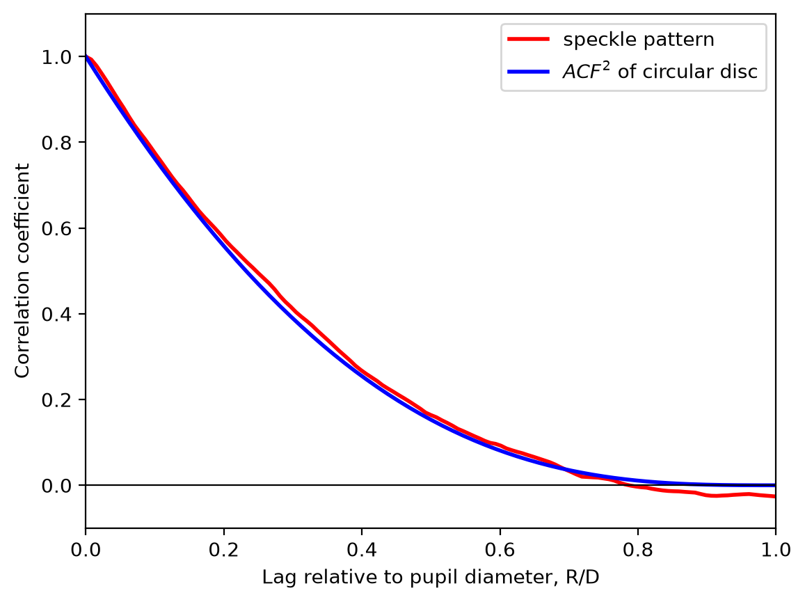
The correlation coefficient has a closed form for this geometry. The speckle correlation is simply the square of the autocorrelation of a circular disc,

\[\mathrm{ACF}(a) = \frac{2}{\pi}\cos^{-1}\left( a - a\sqrt{1-a^2}\right), \qquad \rho = \mathrm{ACF}^2\]

with \(a = R/D\). The measured curve follows it without any fitting.

A single realization wanders a little around the prediction, more so for small images; averaging several realizations converges on it.

lag = np.arange(len(correlation)) / M

plt.plot(lag, correlation, "r-", lw=2, label="speckle pattern")
plt.plot(lag, theory, "b-", lw=2, label="$ACF^2$ of circular disc")
plt.axhline(0, color="black", lw=0.8)
plt.xlabel("Lag relative to pupil diameter, R/D")
plt.ylabel("Correlation coefficient")
plt.axis([0, 1, -0.1, 1.1])
plt.legend()
plt.show()

print("largest departure from theory: %.3f" % np.max(np.abs(correlation - theory)))

largest departure from theory: 0.028

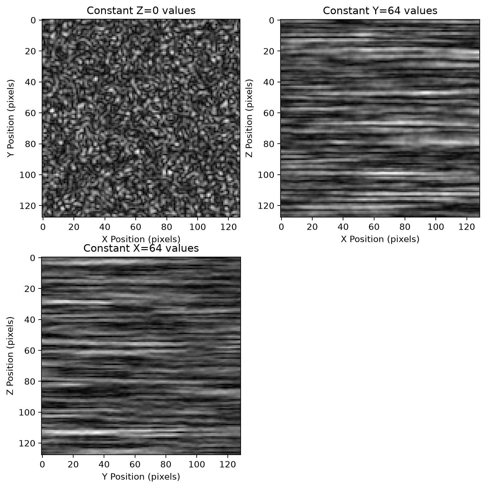
Because the cube is an ordinary three-dimensional array with the frame on its last axis, slice_plot displays it directly. The constant-Z panel is one speckle pattern; the other two are space-time cuts, where the streaks show how long a given point stays bright as the pattern boils.

pyspeckle.slice_plot(cube, M // 2, M // 2, 0)
plt.show()

OCT speckle

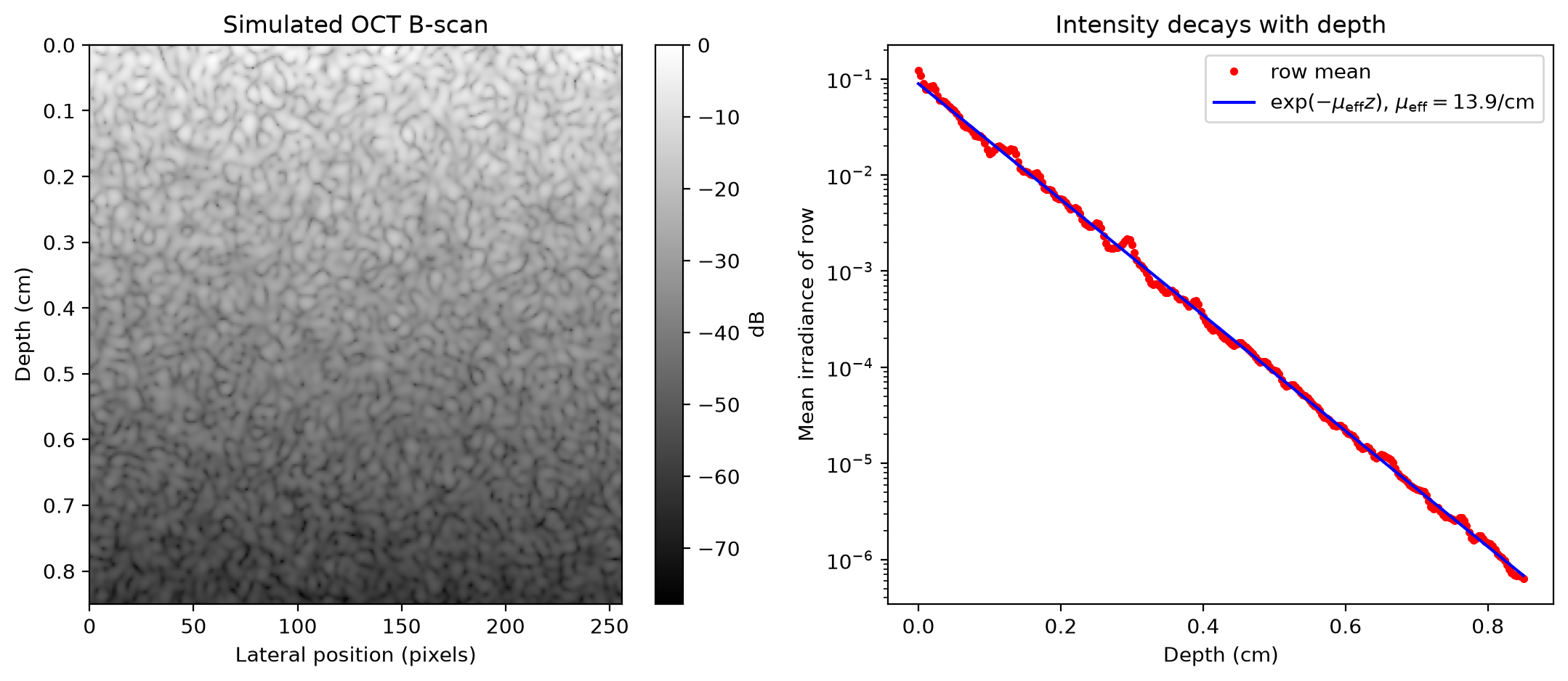
An OCT B-scan is a depth by width image, and its speckle changes with depth. Near the surface the light has scattered once and arrives as a single fully developed pattern, so the contrast is \(K=1\). Deeper down it has scattered many times and arrives as several independent contributions that add in irradiance, which lowers the contrast. At the same time the mean irradiance falls, because the tissue absorbs light and scatters it out of the beam.

create_oct_speckle models the first effect as a degree of polarization that sweeps from one at the surface to zero at the bottom, so the deepest row is exactly the unpolarized pattern with \(K=1/\sqrt{2}\). The second is the diffusion approximation, \(\mu_\mathrm{eff}=\sqrt{3\mu_a(\mu_a+\mu_s')}\). The defaults describe aorta.

mua, musp = 2, 30
image, depth, contrast = pyspeckle.create_oct_speckle((256, 256), 4, mua=mua, musp=musp)
mu_eff = np.sqrt(3 * mua * (mua + musp))

plt.subplots(1, 2, figsize=(13, 5))
plt.subplot(121)
plt.imshow(10 * np.log10(image / image.max()), cmap="gray", aspect="auto", extent=[0, image.shape[1], depth[-1], 0])
plt.colorbar(label="dB")
plt.xlabel("Lateral position (pixels)")
plt.ylabel("Depth (cm)")
plt.title("Simulated OCT B-scan")

plt.subplot(122)
row_mean = image.mean(axis=1)
# anchor the curve to the whole profile, not to one noisy row
scale = np.exp(np.mean(np.log(row_mean) + mu_eff * depth))
plt.semilogy(depth, row_mean, "r.", label="row mean")
plt.semilogy(
    depth,
    scale * np.exp(-mu_eff * depth),
    "b",
    label=r"$\exp(-\mu_\mathrm{eff}z)$, $\mu_\mathrm{eff}=%.1f$/cm" % mu_eff,
)
plt.xlabel("Depth (cm)")
plt.ylabel("Mean irradiance of row")
plt.title("Intensity decays with depth")
plt.legend()

plt.show()

Contrast falls with depth

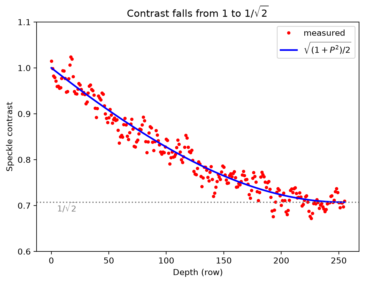
The contrast of each row follows from the two patterns that make it up. With weights \(\frac{1}{2}(1+P)\) and \(\frac{1}{2}(1-P)\) on independent exponential patterns of equal mean,

\[K = \sqrt{\frac{1+P^2}{2}}\]

which create_oct_speckle returns. A single row holds only a few hundred independent speckles, so the measurement is averaged over several patterns.

rows, cols, trials = 256, 512, 8
measured = np.zeros(rows)
for _ in range(trials):
    y, _, contrast = pyspeckle.create_oct_speckle((rows, cols), 4, mua=mua, musp=musp)
    measured += y.std(axis=1) / y.mean(axis=1)
measured /= trials

plt.figure(figsize=(7, 5))
plt.plot(np.arange(rows), measured, "r.", label="measured")
plt.plot(np.arange(rows), contrast, "b", lw=2, label=r"$\sqrt{(1+P^2)/2}$")
plt.axhline(1 / np.sqrt(2), color="gray", ls=":")
plt.text(5, 1 / np.sqrt(2) - 0.02, r"$1/\sqrt{2}$", color="gray")
plt.xlabel("Depth (row)")
plt.ylabel("Speckle contrast")
plt.title("Contrast falls from 1 to $1/\sqrt{2}$")
plt.ylim(0.6, 1.1)
plt.legend()

plt.show()

The irradiance distribution morphs with depth

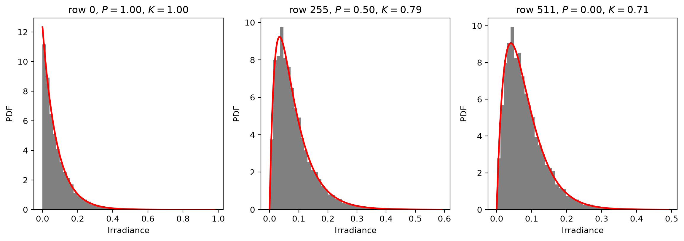
The surface row is a single exponential pattern and the deepest row is the sum of two, which is the gamma-2 distribution of unpolarized speckle. In between the row is a weighted sum of two exponentials with unequal weights, so its density is hypoexponential,

\[f(I)=\frac{\lambda_1\lambda_2}{\lambda_2-\lambda_1} \left(e^{-\lambda_1 I}-e^{-\lambda_2 I}\right), \qquad \lambda_i = \frac{1}{w_i\langle I\rangle}\]

with \(w_1=\frac{1}{2}(1+P)\) and \(w_2=\frac{1}{2}(1-P)\).

def blend_pdf(x, P, mean):
    """Irradiance PDF of a row whose degree of polarization is P."""
    w1, w2 = (1 + P) / 2, (1 - P) / 2
    if w2 < 1e-9:  # one pattern only, so plain exponential
        return np.exp(-x / mean) / mean
    if abs(w1 - w2) < 1e-9:  # equal weights, so gamma-2
        lam = 1 / (w1 * mean)
        return lam**2 * x * np.exp(-lam * x)
    lam1, lam2 = 1 / (w1 * mean), 1 / (w2 * mean)
    return lam1 * lam2 / (lam2 - lam1) * (np.exp(-lam1 * x) - np.exp(-lam2 * x))


rows, chosen = 512, [0, 255, 511]
# one row holds only 512 samples, so pool the same row from several patterns
pooled = {row: [] for row in chosen}
for _ in range(12):
    image, depth, contrast = pyspeckle.create_oct_speckle((rows, 512), 4, mua=0)
    for row in chosen:
        pooled[row].append(image[row])

plt.subplots(1, 3, figsize=(14, 4.2))
for n, row in enumerate(chosen):
    P = 1 - row / (rows - 1)
    values = np.concatenate(pooled[row])
    plt.subplot(1, 3, n + 1)
    plt.hist(values, bins=50, density=True, color="gray")
    g = np.linspace(0, values.max(), 200)
    plt.plot(g, blend_pdf(g, P, values.mean()), "r", lw=2)
    plt.xlabel("Irradiance")
    plt.ylabel("PDF")
    plt.title("row %d, $P=%.2f$, $K=%.2f$" % (row, P, contrast[row]))

plt.show()

Local contrast

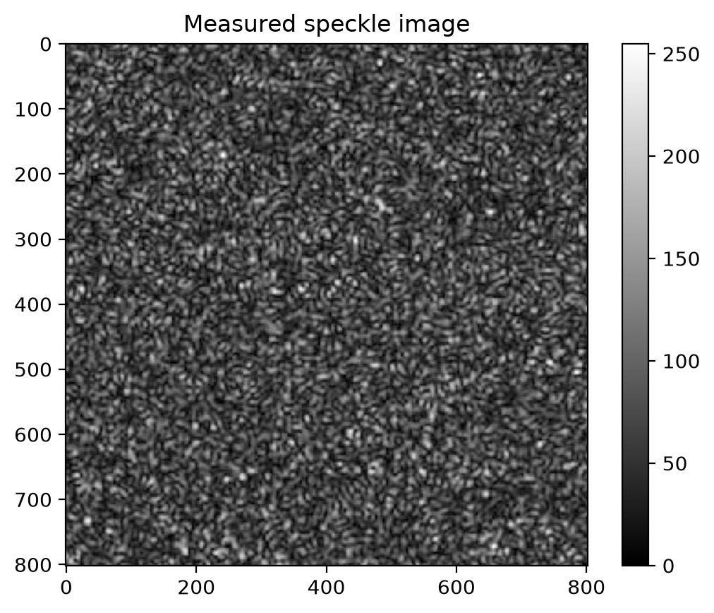
Speckle contrast is often measured over a sliding window rather than over a whole image, because the window can follow variation across a scene. local_contrast_2D correlates the pattern with a kernel and returns the contrast at every valid position, together with the contrast of the whole image.

Here it is applied to a measured speckle image rather than a simulated one.

im = imageio.v2.imread(repo + "speckle.png")
plt.imshow(im, cmap="gray")
plt.colorbar()
plt.title("Measured speckle image")
plt.show()

kernel = np.ones((10, 10))
pyspeckle.local_contrast_plot(im, kernel)
# no theory curve on the irradiance panel: this is a measured image, not a
# generated one, and its contrast of about 0.46 shows it is not fully developed
plt.subplot(224)
C, _ = pyspeckle.local_contrast(im, kernel)
c = np.linspace(C.min(), C.max(), 200)
plt.plot(c, np.exp(-((c - C.mean()) ** 2) / (2 * C.std() ** 2)) / (C.std() * np.sqrt(2 * np.pi)), "r", lw=2)

plt.show()

Summary

• the aperture sets the speckle size and shape; pix_per_speckle, alpha, and shape all act through it

• create_exponential gives fully developed polarized speckle with exponential irradiance and contrast 1

• create_unpolarized gives contrast \(1/\sqrt{2}\)

• create_phase_screen provides the rough-surface phase needed for partially developed speckle

• create_boiling_speckle produces a decorrelating sequence, with the correlation coefficient and its theoretical prediction

• local_contrast_2D and local_contrast_plot measure contrast over a sliding window