2D Speckle Generation & Analysis

Scott Prahl

Aug 2023

Adapted from the SimSpeckle Matlab script package described in Donald D. Duncan, Sean J. Kirkpatrick, “Algorithms for simulation of speckle (laser and otherwise),” Proc. SPIE 6855, Complex Dynamics and Fluctuations in Biomedical Photonics V, 685505 (6 February 2008); https://doi.org/10.1117/12.760518

A PDF is available at https://www.researchgate.net/profile/Sean-Kirkpatrick-2/publication/233783056_Algorithms_for_simulation_of_speckle_laser_and_otherwise/links/09e4150b78c4e8fe5f000000/Algorithms-for-simulation-of-speckle-laser-and-otherwise.pdf

import imageio
import numpy as np
import matplotlib.pyplot as plt
import pyspeckle

%config InlineBackend.figure_format='retina'

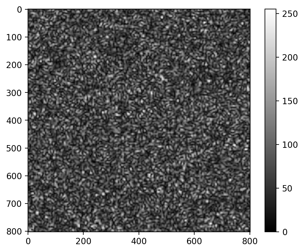
Test image

im = imageio.v2.imread('https://omlc.org/~prahl/host/453/week5/speckle.png')
plt.imshow(im, cmap='gray')
plt.colorbar()
plt.show()

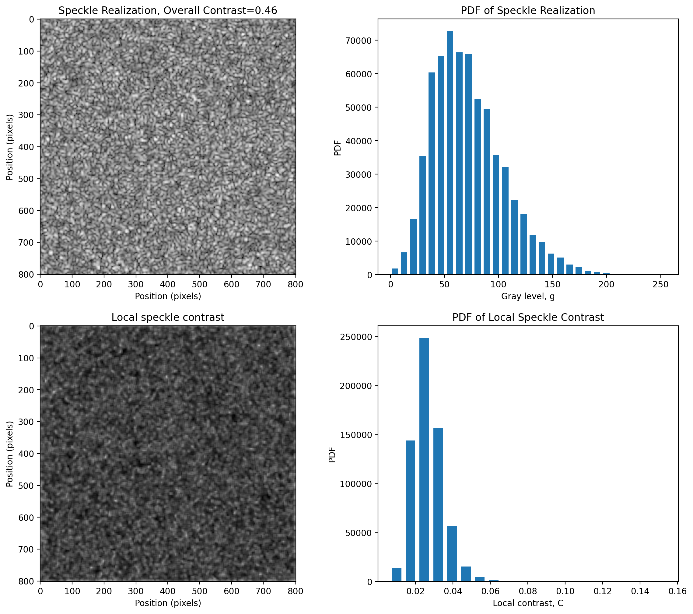
Local Contrast

\[z[k] = (x * y)(k - N + 1) = \sum_{l=0}^{||x||-1}x_l y_{l-k+N-1}^{*}\]

kernel=np.ones((10,10))
pyspeckle.local_contrast_2D_plot(im,kernel)
plt.show()

Exponential Speckle

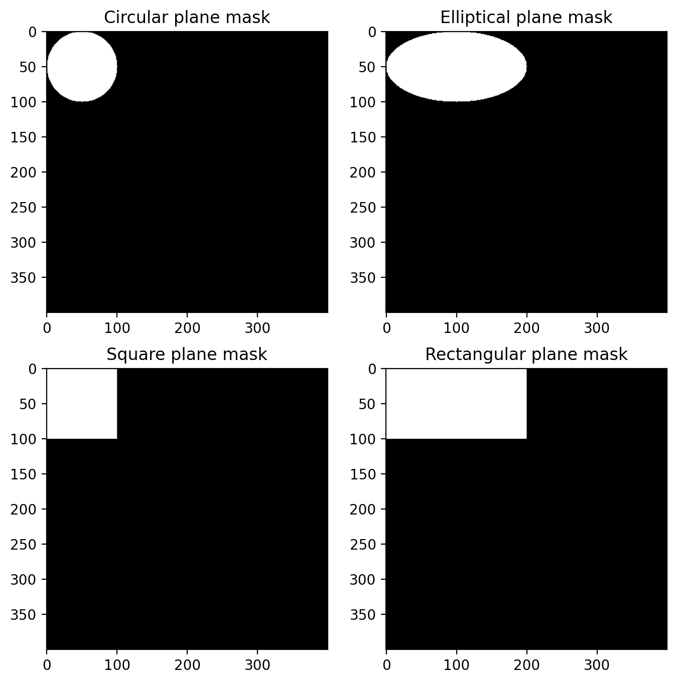
Masks used internally

These routines won’t typically be called directly, but are used internally to create speckle. These routines are not exported by default and all begin with an underscore ‘_’.

This just shows that the function is working as expected.

#import pyspeckle.pyspeckle
L=100
pix_per_speckle=4
N = pix_per_speckle * L
R = int(L/2)

plt.subplots(2,2, figsize=(8,8))
plt.subplot(2,2,1)
mask = pyspeckle.pyspeckle._create_mask(N,R,R)
plt.imshow(mask,cmap='gray')
plt.title('Circular plane mask')

plt.subplot(2,2,2)
mask = pyspeckle.pyspeckle._create_mask(N,L,R)
plt.imshow(mask,cmap='gray')
plt.title('Elliptical plane mask')

plt.subplot(2,2,3)
mask = pyspeckle.pyspeckle._create_mask(N,R,R,shape='square')
plt.imshow(mask,cmap='gray')
plt.title('Square plane mask')

plt.subplot(2,2,4)
mask = pyspeckle.pyspeckle._create_mask(N,L,R,shape='square')
plt.imshow(mask,cmap='gray')
plt.title('Rectangular plane mask')

plt.show()

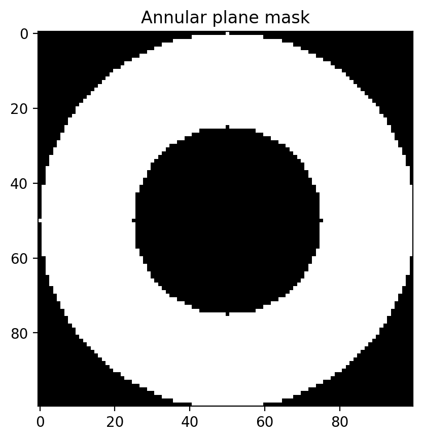
L=50
pix_per_speckle=2
N = pix_per_speckle * L
R = int(L/2)

mask = pyspeckle.pyspeckle._create_mask(N,R,L,shape='annulus')
plt.imshow(mask,cmap='gray')
plt.title('Annular plane mask')
plt.show()

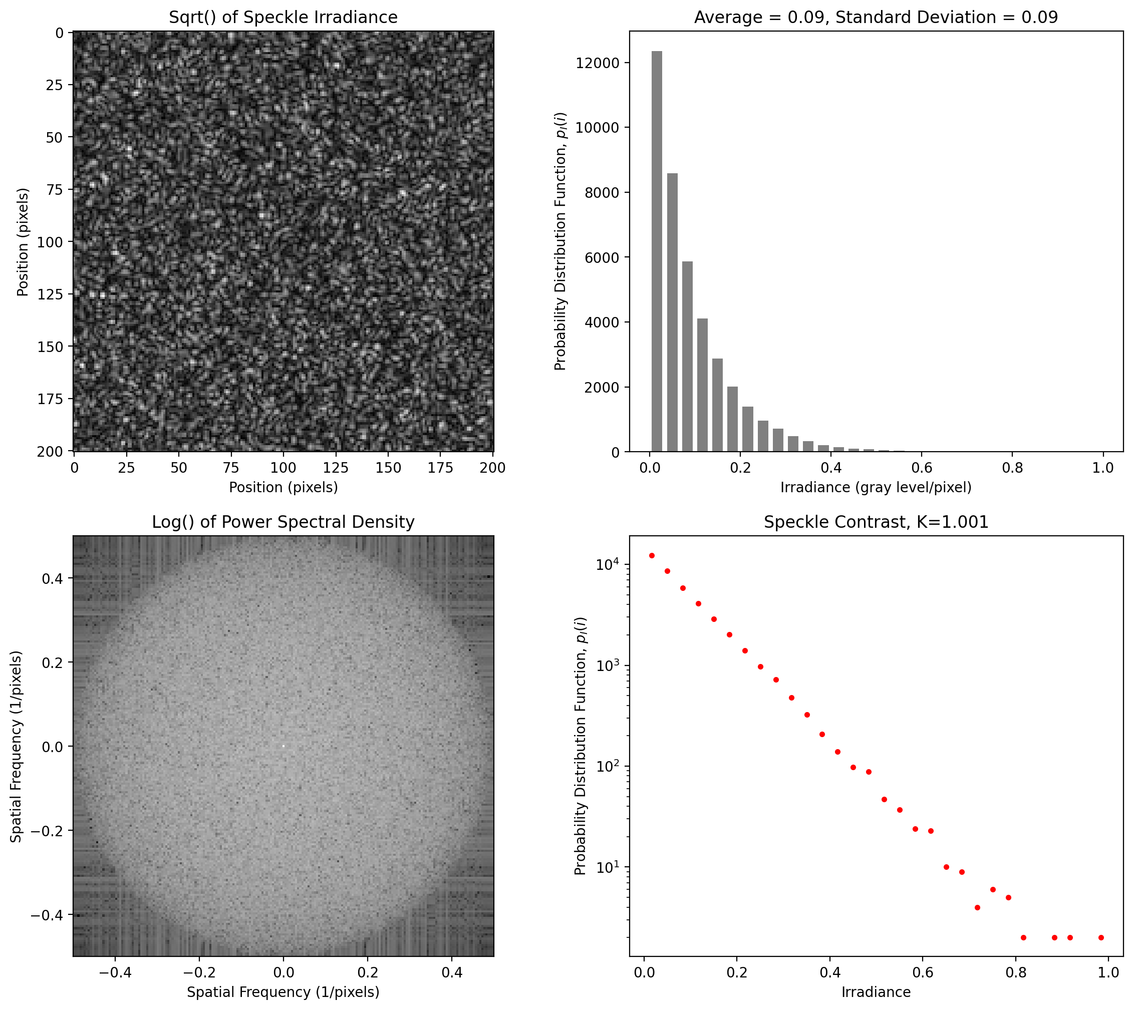
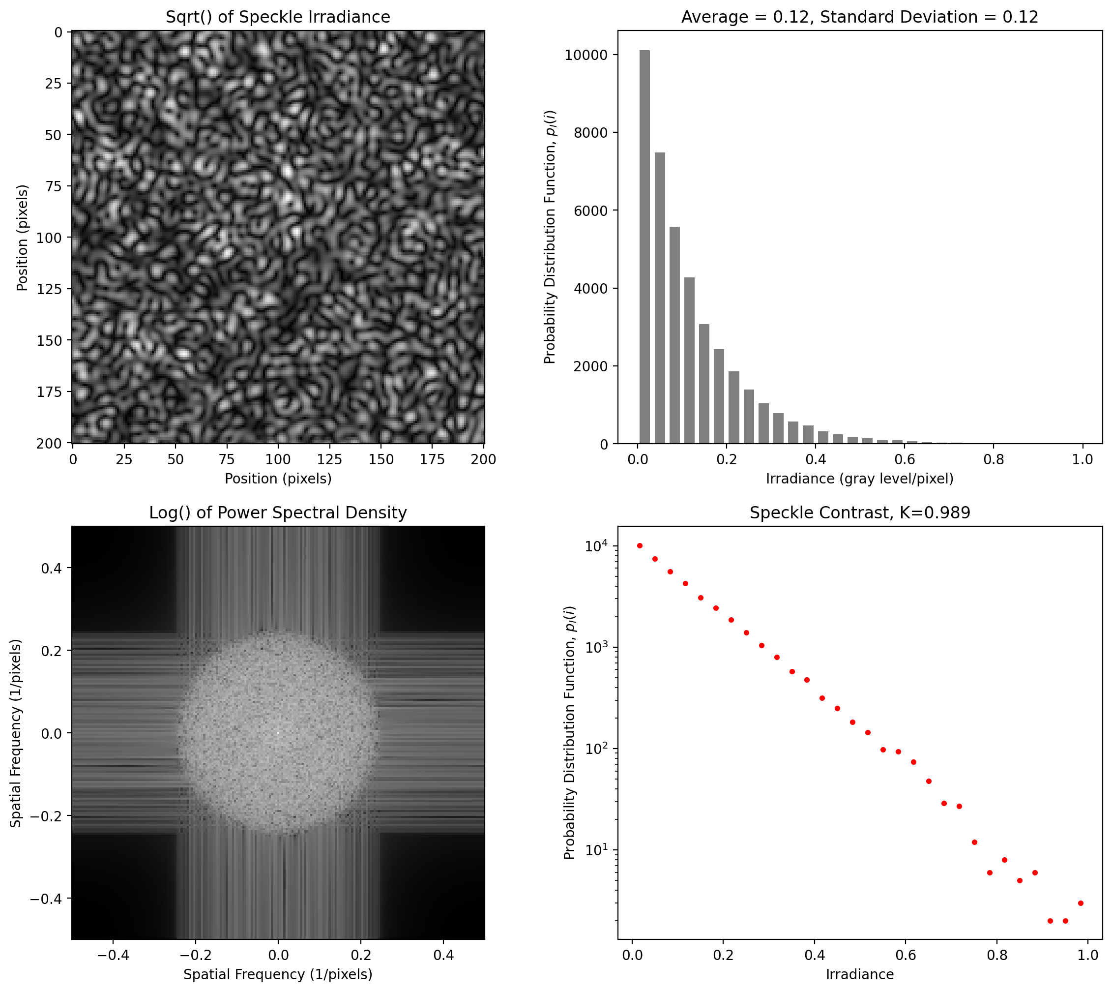
Isotropic Speckle at Nyquist Limit (2 pixels per smallest pixel)

This speckle pattern has an exponential probability distribution function that is spatially bandwidth-limited by the specified pixels per speckle. The statistics are uniform in all directions.

The Power Spectral Density can be used to establish the dimensions of the minimum speckle size. When the display reaches the edge of the image, the speckle pattern (in that dimension) is at Nyquist, i.e., two pixels per (minimum) speckle. This is what we observe here.

y = pyspeckle.create_Exponential(201,2)
pyspeckle.statistics_plot(y)
#plt.savefig('twoD_speckle.png', dpi=300)
plt.show()

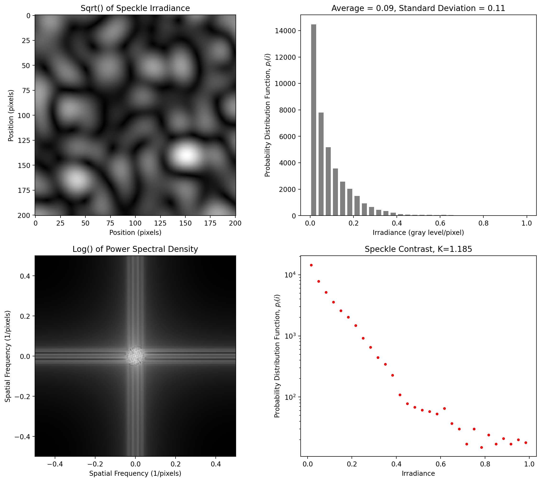
Isotropic Speckle at 4 pixels per smallest pixel

y = pyspeckle.create_Exponential(201,20)
pyspeckle.statistics_plot(y)

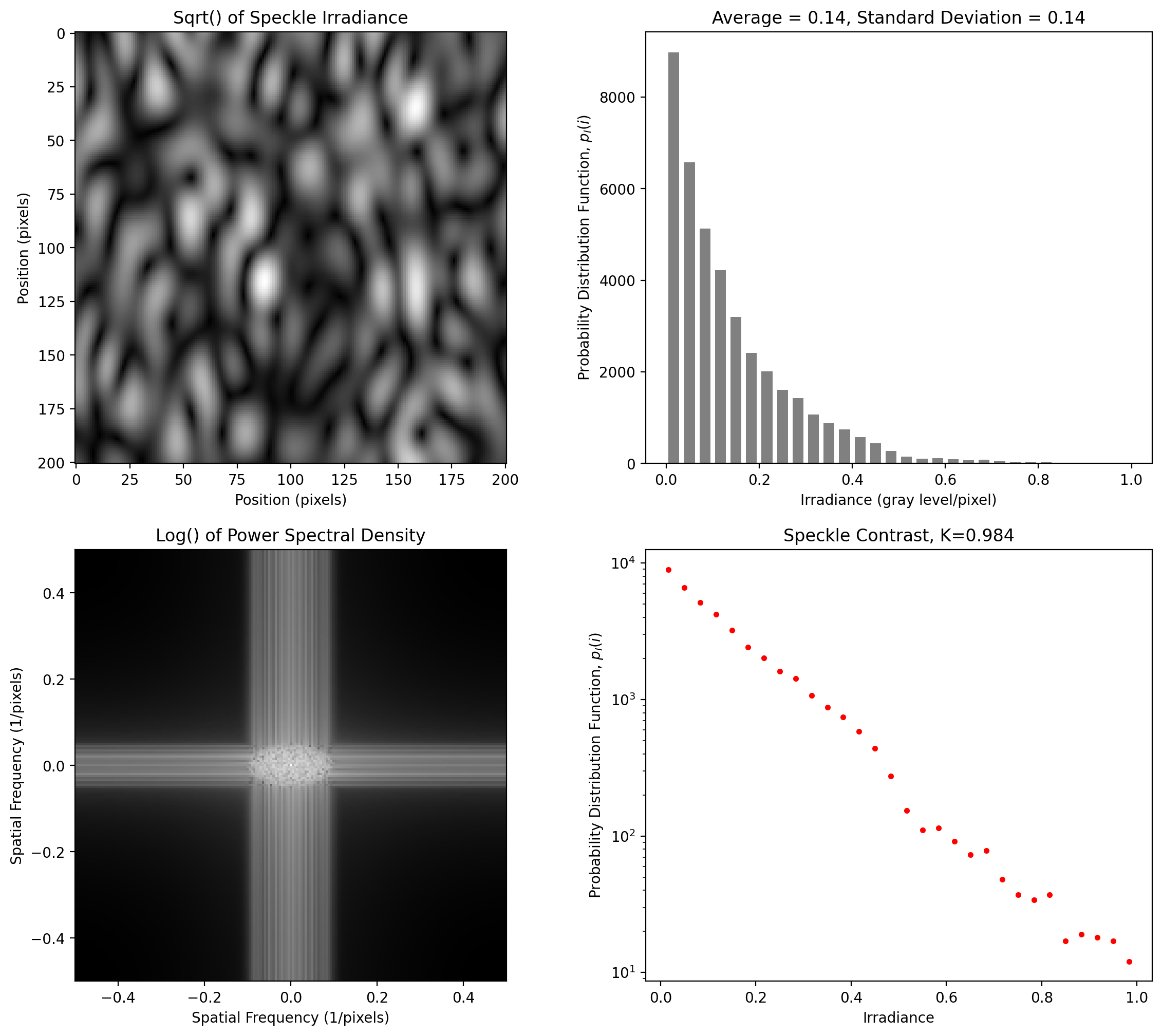
Elliptical Speckle at 4 pixels per smallest pixel

y = pyspeckle.create_Exponential(201,10,alpha=0.5)
pyspeckle.statistics_plot(y)

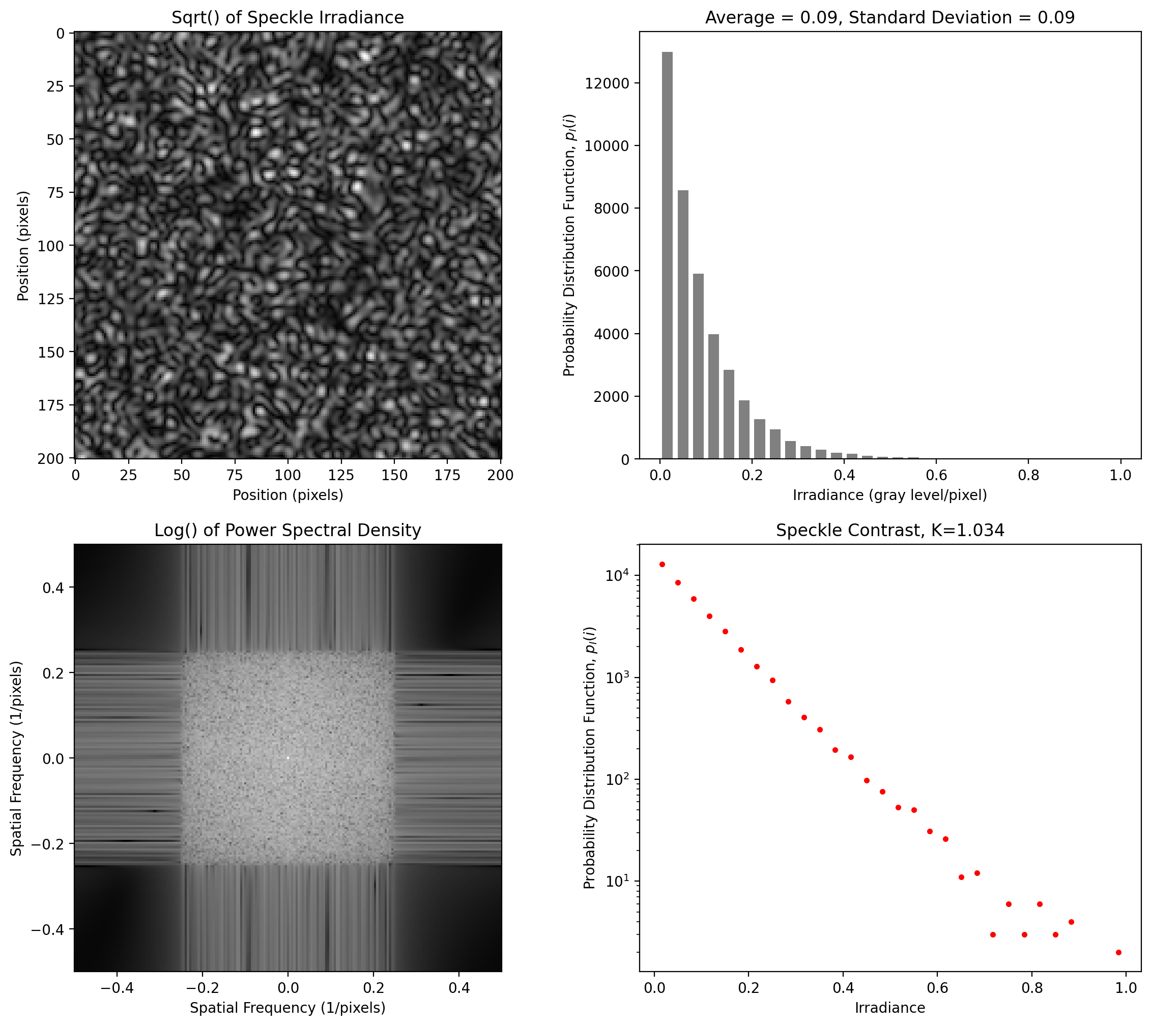
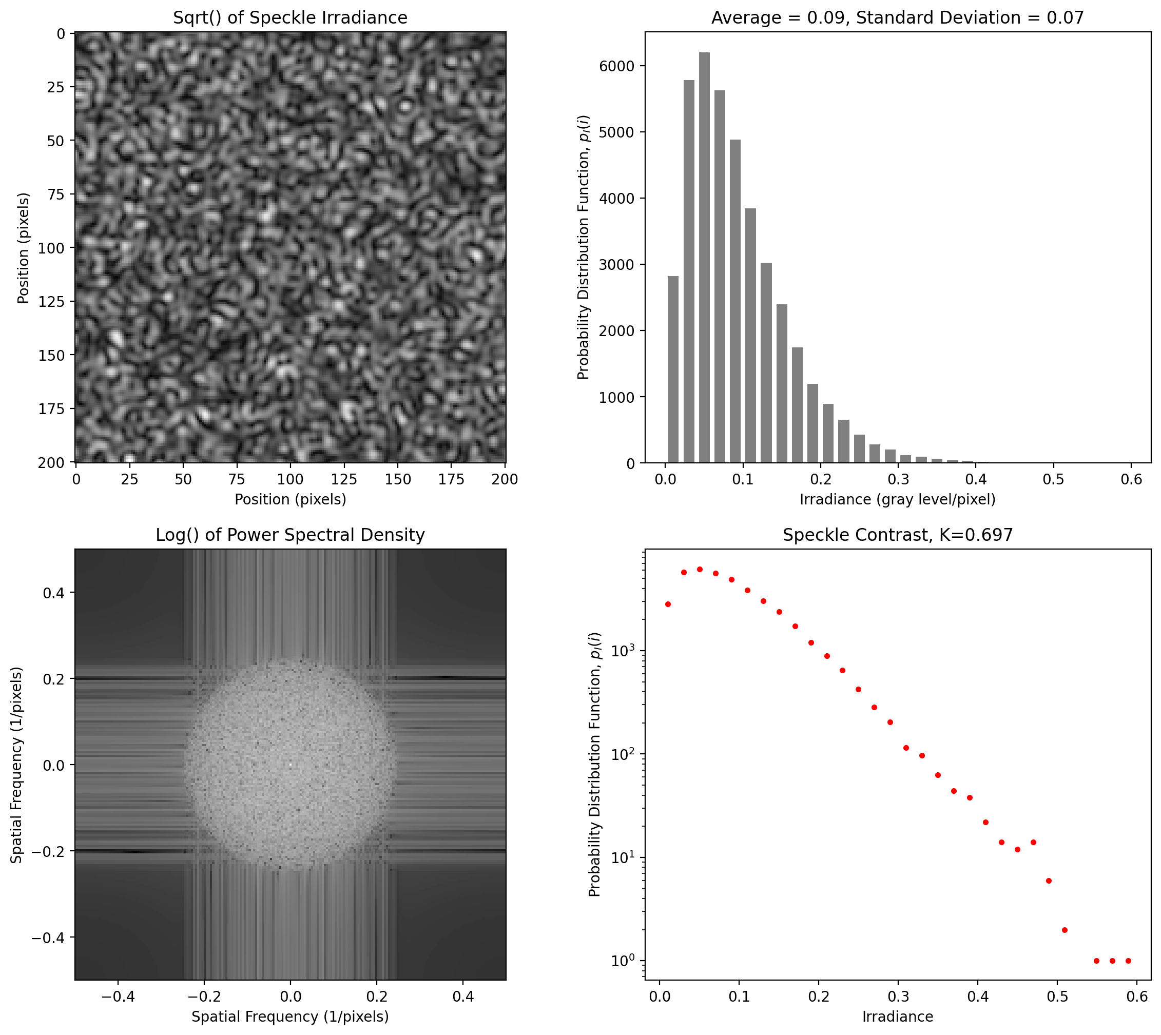
Near-Isotropic Speckle at 4 pixels per smallest pixel

y = pyspeckle.create_Exponential(201,4,shape='square')
pyspeckle.statistics_plot(y)

Polarized Speckle for annular spot

y = pyspeckle.create_Exponential(201,4,shape='annulus',alpha=3)
pyspeckle.statistics_plot(y)

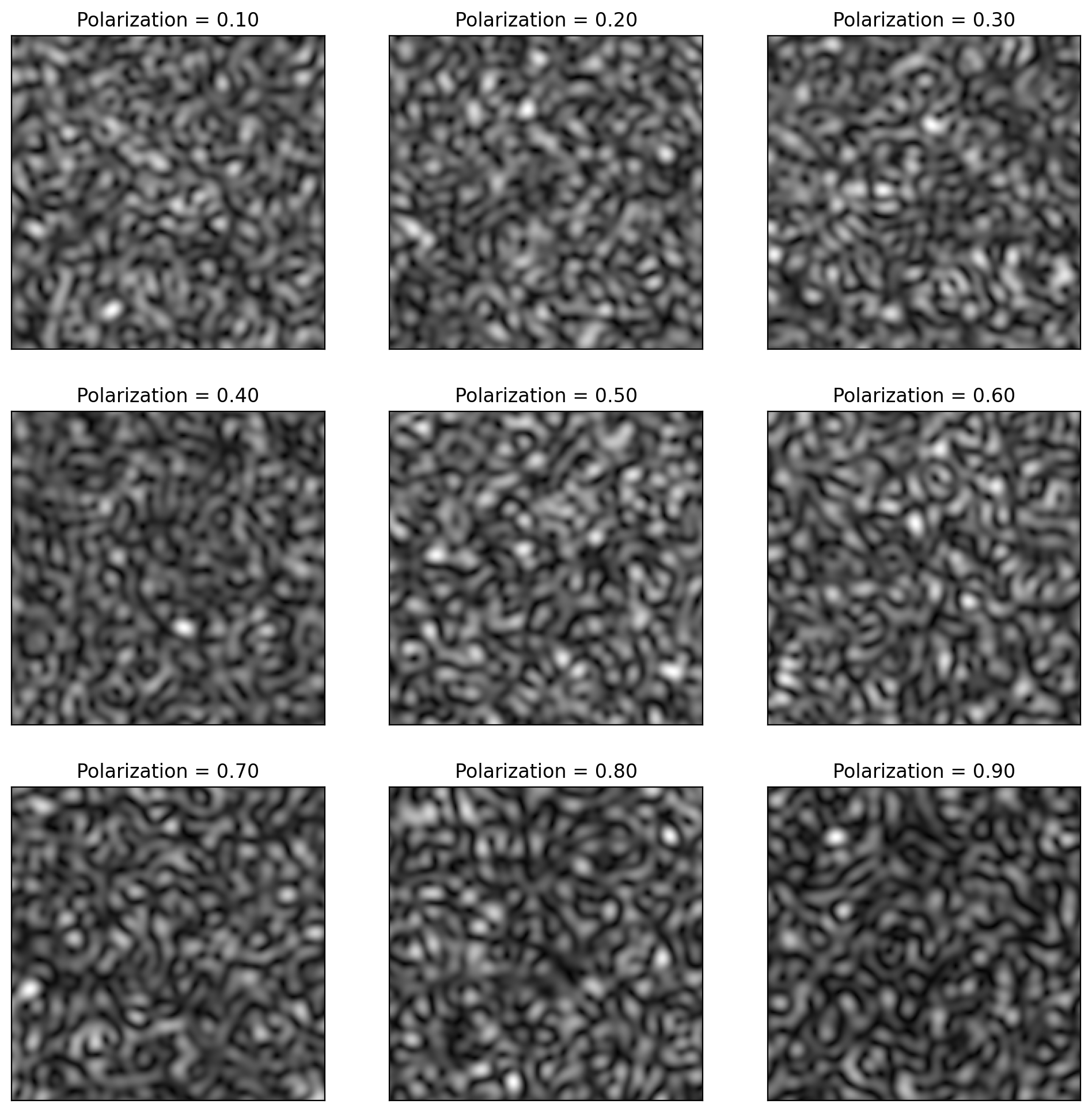
Speckle for Polarized light

Varies by degree of polarization

y = pyspeckle.create_Exponential(201,4,polarization=0.1)
pyspeckle.statistics_plot(y)

plt.subplots(3,3,figsize=(12,12))
for i,pol in enumerate([0.1,0.2,0.3,0.4,0.5,0.6,0.7,0.8,0.9]):
    plt.subplot(3,3,i+1)
    y = pyspeckle.create_Exponential(201,8,polarization=pol)
    plt.imshow(np.sqrt(y),cmap='gray')
    plt.title('Polarization = %.2f'%pol)
    plt.xticks([])
    plt.yticks([])

plt.show()

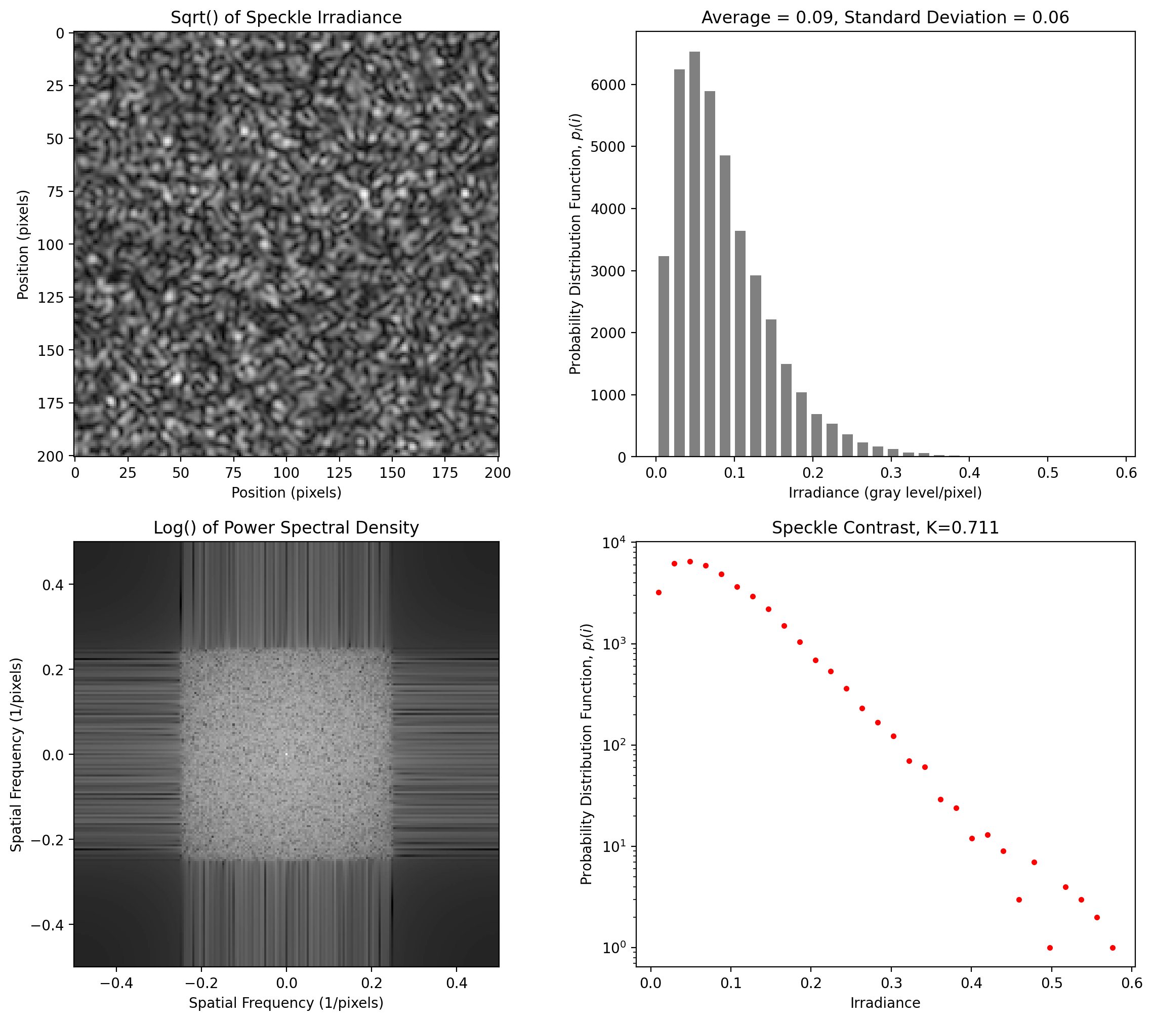
Unpolarized Speckle

This arises from adding two speckle patterns (one for each polarization state). The result is a pattern with a Rayleigh intensity distribution

y = pyspeckle.create_Rayleigh(201,4,shape='square')
pyspeckle.statistics_plot(y)