3D Speckle Generation & Analysis
Scott Prahl
September 2023
Adapted from the SimSpeckle Matlab script package described in Donald D. Duncan, Sean J. Kirkpatrick, “Algorithms for simulation of speckle (laser and otherwise),” Proc. SPIE 6855, Complex Dynamics and Fluctuations in Biomedical Photonics V, 685505 (6 February 2008); https://doi.org/10.1117/12.760518
[1]:
%config InlineBackend.figure_format = 'retina'

import sys
import numpy as np
import matplotlib.pyplot as plt

if sys.platform == "emscripten":
    import piplite

    await piplite.install("pyspeckle")

import pyspeckle
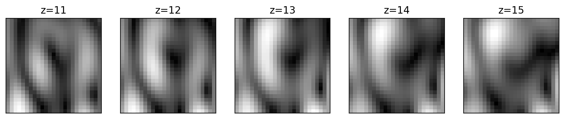
Create simple 3D speckle image
Generate an 25 x 25 x 25 polarized, fully-developed speckle irradiance pattern.
The speckle pattern will have an exponential probability distribution function that is spatially bandwidth-limited by the specified pixels per speckle.
The resolution is specified by the parameter pix_per_speckle and refers to the smallest speckle size. Thus pix_per_speckle=5 will have five pixels across the smallest speckle.
Non-circular speckle is supported using alpha and beta. This is defined as the ratio of x-speckle size to y-speckle size (or x to z). alpha=2 will have speckles that with y-dimensions that are twice the x-dimension. Similarly beta=2 will have speckles that with z-dimensions that are twice the x-dimension.
[2]:
x = pyspeckle.create_Exponential_3D(25, 5, alpha=2, beta=2)
y = np.sqrt(x)
[3]:
def showone(i):
    plt.subplot(1, 5, i)
    j = 10 + i
    plt.imshow(y[:, :, j], cmap="gray")
    plt.xticks([])
    plt.yticks([])
    plt.title("z=%i" % j)


plt.subplots(1, 5, figsize=(12, 4))
for i in range(1, 6):
    showone(i)
plt.show()
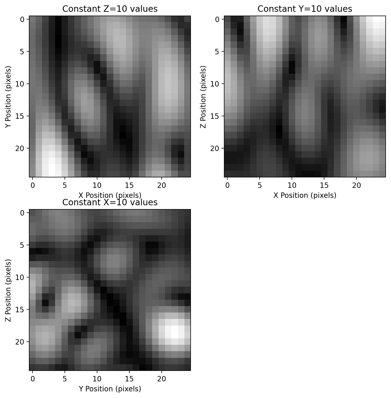
[4]:
plt.figure(figsize=(10, 10))
pyspeckle.slice_plot(x, 10, 10, 10)
plt.show()
<Figure size 1000x1000 with 0 Axes>
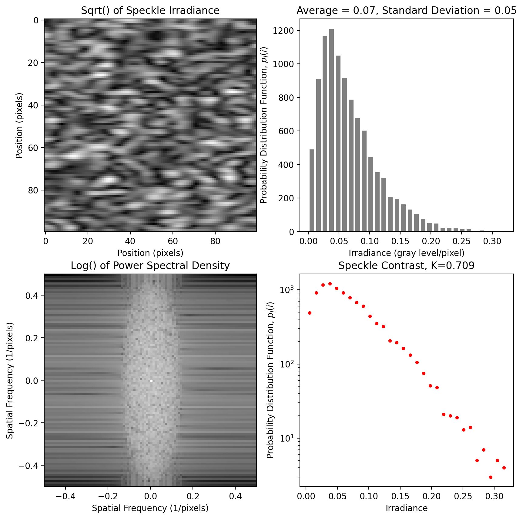
Unpolarized (Rayleigh) Speckle
[5]:
x = pyspeckle.create_Exponential_3D(100, 2, alpha=0.3, polarization=0.0)
y = np.sqrt(x)
and look at the statistics for a slice of the cube for z=50
[6]:
plt.figure(figsize=(10, 10))
pyspeckle.statistics_plot(x[:, :, 50], initialize=False)
plt.show()